Machine Learning Mastery 生成对抗网络教程(四)
原文:Machine Learning Mastery协议:CC BY-NC-SA 4.0如何开发用于图像到图像转换的 Pix2Pix GAN原文:https://machinelearningmastery.com/how-to-develop-a-pix2pix-gan-for-image-to-image-translation/最后更新于 2021 年 1 月 18 日Pix2Pix 生成
如何开发用于图像到图像转换的 Pix2Pix GAN
原文:https://machinelearningmastery.com/how-to-develop-a-pix2pix-gan-for-image-to-image-translation/
最后更新于 2021 年 1 月 18 日
Pix2Pix 生成对抗网络是一种训练深度卷积神经网络的方法,用于图像到图像的翻译任务。
作为一种有图像条件的 GAN,架构的精心配置允许与现有的 GAN 模型(例如 256×256 像素)相比生成大图像,并且能够在各种不同的图像到图像转换任务中表现良好。
在本教程中,您将发现如何为图像到图像的翻译开发一个 Pix2Pix 生成式对抗网络。
完成本教程后,您将知道:
- 如何将卫星图像加载并准备到谷歌地图图像到图像转换数据集。
- 如何开发一个 Pix2Pix 模型,用于将卫星照片翻译成谷歌地图图像。
- 如何使用最终的 Pix2Pix 生成器模型来翻译临时卫星图像。
用我的新书Python 生成对抗网络启动你的项目,包括分步教程和所有示例的 Python 源代码文件。
我们开始吧。
- 2021 年 1 月更新:更新所以层冻结用批量定额。
如何开发用于图像到图像转换的 Pix2Pix 生成对抗网络
图片由欧洲南方天文台提供,保留部分权利。
教程概述
本教程分为五个部分;它们是:
- 什么是 Pix2Pix GAN?
- 卫星到地图图像转换数据集
- 如何开发和训练 Pix2Pix 模型
- 如何使用 Pix2Pix 模型翻译图像
- 如何将谷歌地图翻译成卫星图像
什么是 Pix2Pix GAN?
Pix2Pix 是一个为通用图像到图像转换而设计的生成对抗网络模型。
这种方法是由菲利普·伊索拉等人在 2016 年发表的论文《条件对抗网络下的 T2 图像到图像转换》和 2017 年在 CVPR 发表的《T4》中提出的。
GAN 架构由一个用于输出新的似是而非的合成图像的生成器模型和一个将图像分类为真实(来自数据集)或虚假(生成)的鉴别器模型组成。鉴别器模型直接更新,而生成器模型通过鉴别器模型更新。这样,两个模型在对抗过程中被同时训练,其中生成器试图更好地欺骗鉴别器,鉴别器试图更好地识别伪造图像。
Pix2Pix 模型是一种条件 GAN 或 cGAN,其中输出图像的生成取决于输入,在这种情况下是源图像。鉴别器同时具有源图像和目标图像,并且必须确定目标是否是源图像的似是而非的变换。
生成器通过对抗性损失进行训练,这鼓励生成器在目标域中生成似是而非的图像。生成器还通过在生成的图像和预期输出图像之间测量的 L1 损耗来更新。这种额外的损失促使生成器模型创建源图像的似是而非的翻译。
Pix2Pix GAN 已经在一系列图像到图像的转换任务中进行了演示,例如将地图转换为卫星照片,将黑白照片转换为彩色照片,以及将产品草图转换为产品照片。
现在我们已经熟悉了 Pix2Pix GAN,让我们准备一个数据集,可以用于图像到图像的转换。
卫星到地图图像转换数据集
在本教程中,我们将使用 Pix2Pix 论文中使用的所谓的“地图”数据集。
这是一个由纽约卫星图像和相应的谷歌地图页面组成的数据集。图像转换问题涉及将卫星照片转换为谷歌地图格式,或者相反,将谷歌地图图像转换为卫星照片。
该数据集在 pix2pix 网站上提供,可以作为 255 兆字节的 zip 文件下载。
下载数据集并将其解压缩到当前工作目录中。这将创建一个名为“地图”的目录,其结构如下:
maps
├── train
└── val
train 文件夹包含 1,097 个图像,而验证数据集包含 1,099 个图像。
图像有一个数字文件名,并且是 JPEG 格式。每幅图像宽 1200 像素,高 600 像素,左侧包含卫星图像,右侧包含谷歌地图图像。
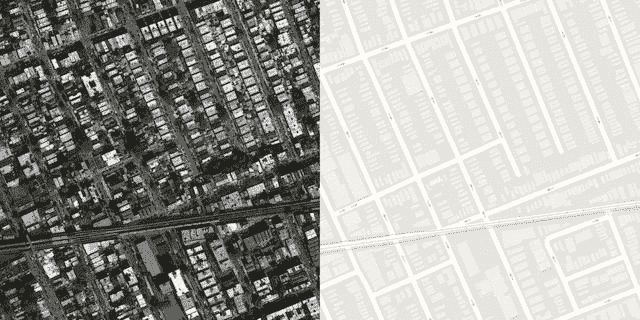
地图数据集中的样本图像,包括卫星和谷歌地图图像。
我们可以准备这个数据集,在 Keras 训练一个 Pix2Pix GAN 模型。我们将只处理训练数据集中的图像。每张图片都将被加载、重新缩放,并分割成卫星和谷歌地图元素。结果将是 1097 个彩色图像对,宽度和高度为 256×256 像素。
下面的 load_images() 函数实现了这一点。它枚举给定目录中的图像列表,加载每个目标大小为 256×512 像素的图像,将每个图像拆分为卫星和地图元素,并返回每个元素的数组。
# load all images in a directory into memory
def load_images(path, size=(256,512)):
	src_list, tar_list = list(), list()
	# enumerate filenames in directory, assume all are images
	for filename in listdir(path):
		# load and resize the image
		pixels = load_img(path + filename, target_size=size)
		# convert to numpy array
		pixels = img_to_array(pixels)
		# split into satellite and map
		sat_img, map_img = pixels[:, :256], pixels[:, 256:]
		src_list.append(sat_img)
		tar_list.append(map_img)
	return [asarray(src_list), asarray(tar_list)]
我们可以用训练数据集的路径调用这个函数。加载后,我们可以将准备好的数组保存到一个新的压缩格式的文件中,供以后使用。
下面列出了完整的示例。
# load, split and scale the maps dataset ready for training
from os import listdir
from numpy import asarray
from numpy import vstack
from keras.preprocessing.image import img_to_array
from keras.preprocessing.image import load_img
from numpy import savez_compressed

# load all images in a directory into memory
def load_images(path, size=(256,512)):
	src_list, tar_list = list(), list()
	# enumerate filenames in directory, assume all are images
	for filename in listdir(path):
		# load and resize the image
		pixels = load_img(path + filename, target_size=size)
		# convert to numpy array
		pixels = img_to_array(pixels)
		# split into satellite and map
		sat_img, map_img = pixels[:, :256], pixels[:, 256:]
		src_list.append(sat_img)
		tar_list.append(map_img)
	return [asarray(src_list), asarray(tar_list)]

# dataset path
path = 'maps/train/'
# load dataset
[src_images, tar_images] = load_images(path)
print('Loaded: ', src_images.shape, tar_images.shape)
# save as compressed numpy array
filename = 'maps_256.npz'
savez_compressed(filename, src_images, tar_images)
print('Saved dataset: ', filename)
运行该示例将加载训练数据集中的所有图像,总结它们的形状以确保图像被正确加载,然后以压缩的 NumPy 数组格式将数组保存到名为 maps_256.npz 的新文件中。
Loaded:  (1096, 256, 256, 3) (1096, 256, 256, 3)
Saved dataset:  maps_256.npz
稍后可以通过 load() NumPy 函数依次检索每个数组来加载该文件。
然后,我们可以绘制一些图像对,以确认数据已被正确处理。
# load the prepared dataset
from numpy import load
from matplotlib import pyplot
# load the dataset
data = load('maps_256.npz')
src_images, tar_images = data['arr_0'], data['arr_1']
print('Loaded: ', src_images.shape, tar_images.shape)
# plot source images
n_samples = 3
for i in range(n_samples):
	pyplot.subplot(2, n_samples, 1 + i)
	pyplot.axis('off')
	pyplot.imshow(src_images[i].astype('uint8'))
# plot target image
for i in range(n_samples):
	pyplot.subplot(2, n_samples, 1 + n_samples + i)
	pyplot.axis('off')
	pyplot.imshow(tar_images[i].astype('uint8'))
pyplot.show()
运行此示例加载准备好的数据集并总结每个数组的形状,这证实了我们对 10256×256 个图像对的期望。
Loaded: (1096, 256, 256, 3) (1096, 256, 256, 3)
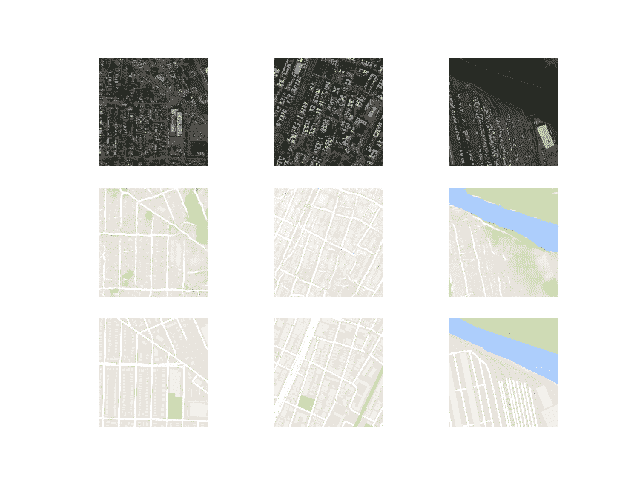
还创建了三个图像对的图,在顶部显示卫星图像,在底部显示谷歌地图图像。
我们可以看到,卫星图像非常复杂,尽管谷歌地图图像简单得多,但它们对主要道路、水和公园等有颜色编码。

显示卫星图像(上)和谷歌地图图像(下)的三对图像图。
现在我们已经为图像转换准备了数据集,我们可以开发我们的 Pix2Pix GAN 模型了。
如何开发和训练 Pix2Pix 模型
在本节中,我们将开发 Pix2Pix 模型,用于将卫星照片翻译成谷歌地图图像。
论文中描述的相同模型架构和配置被用于一系列图像转换任务。该架构在论文正文中有所描述,在论文附录中有更多的细节,并且提供了一个完全工作的实现作为 Torch 深度学习框架的开源。
本节中的实现将使用 Keras 深度学习框架,该框架直接基于本文中描述的模型,并在作者的代码库中实现,旨在拍摄和生成大小为 256×256 像素的彩色图像。
该架构由两个模型组成:鉴别器和生成器。
鉴别器是执行图像分类的深度卷积神经网络。具体来说,条件图像分类。它将源图像(例如卫星照片)和目标图像(例如谷歌地图图像)都作为输入,并预测目标图像是真实的还是源图像的假翻译的可能性。
鉴别器的设计基于模型的有效感受野,它定义了模型的一个输出与输入图像中的像素数之间的关系。这被称为 PatchGAN 模型,经过精心设计,模型的每个输出预测都映射到输入图像的 70×70 的正方形或面片。这种方法的好处是相同的模型可以应用于不同尺寸的输入图像,例如大于或小于 256×256 像素。
模型的输出取决于输入图像的大小,但可能是一个值或值的平方激活图。每一个值都是输入图像中的一个补丁是真实的可能性的概率。如果需要,可以对这些值进行平均,以给出总体可能性或分类分数。
下面的 define_discriminator() 函数按照文中模型的设计实现了 70×70 的 PatchGAN 鉴别器模型。该模型采用两个连接在一起的输入图像,并预测预测的补丁输出。使用二进制交叉熵优化模型,并使用权重,使得模型的更新具有通常效果的一半(0.5)。Pix2Pix 的作者推荐这种模型更新的权重,以减缓训练期间相对于生成器模型的鉴别器变化。
# define the discriminator model
def define_discriminator(image_shape):
	# weight initialization
	init = RandomNormal(stddev=0.02)
	# source image input
	in_src_image = Input(shape=image_shape)
	# target image input
	in_target_image = Input(shape=image_shape)
	# concatenate images channel-wise
	merged = Concatenate()([in_src_image, in_target_image])
	# C64
	d = Conv2D(64, (4,4), strides=(2,2), padding='same', kernel_initializer=init)(merged)
	d = LeakyReLU(alpha=0.2)(d)
	# C128
	d = Conv2D(128, (4,4), strides=(2,2), padding='same', kernel_initializer=init)(d)
	d = BatchNormalization()(d)
	d = LeakyReLU(alpha=0.2)(d)
	# C256
	d = Conv2D(256, (4,4), strides=(2,2), padding='same', kernel_initializer=init)(d)
	d = BatchNormalization()(d)
	d = LeakyReLU(alpha=0.2)(d)
	# C512
	d = Conv2D(512, (4,4), strides=(2,2), padding='same', kernel_initializer=init)(d)
	d = BatchNormalization()(d)
	d = LeakyReLU(alpha=0.2)(d)
	# second last output layer
	d = Conv2D(512, (4,4), padding='same', kernel_initializer=init)(d)
	d = BatchNormalization()(d)
	d = LeakyReLU(alpha=0.2)(d)
	# patch output
	d = Conv2D(1, (4,4), padding='same', kernel_initializer=init)(d)
	patch_out = Activation('sigmoid')(d)
	# define model
	model = Model([in_src_image, in_target_image], patch_out)
	# compile model
	opt = Adam(lr=0.0002, beta_1=0.5)
	model.compile(loss='binary_crossentropy', optimizer=opt, loss_weights=[0.5])
	return model
生成器模型比鉴别器模型更复杂。
生成器是一个使用 U-Net 架构的编码器-解码器模型。该模型获取源图像(例如卫星照片)并生成目标图像(例如谷歌地图图像)。它通过首先将输入图像向下采样或编码到瓶颈层,然后将瓶颈表示向上采样或解码到输出图像的大小来实现这一点。U-Net 架构意味着在编码层和相应的解码层之间增加了跳跃连接,形成一个 U 形。
下图清楚地显示了跳过连接,显示了编码器的第一层是如何连接到解码器的最后一层的,以此类推。

基于条件对抗网络的图像到图像转换的 U-Net 生成器模型架构
生成器的编码器和解码器由卷积的标准化块、批处理标准化、丢弃和激活层组成。这种标准化意味着我们可以开发助手函数来创建每个层块,并重复调用它来构建模型的编码器和解码器部分。
下面的 define_generator() 函数实现了 U-Net 编解码生成器模型。它使用*定义 _ 编码器 _ 块()辅助函数为编码器创建层块,使用解码器 _ 块()*函数为解码器创建层块。tanh 激活函数用于输出层,这意味着生成的图像中的像素值将在[-1,1]的范围内。
# define an encoder block
def define_encoder_block(layer_in, n_filters, batchnorm=True):
	# weight initialization
	init = RandomNormal(stddev=0.02)
	# add downsampling layer
	g = Conv2D(n_filters, (4,4), strides=(2,2), padding='same', kernel_initializer=init)(layer_in)
	# conditionally add batch normalization
	if batchnorm:
		g = BatchNormalization()(g, training=True)
	# leaky relu activation
	g = LeakyReLU(alpha=0.2)(g)
	return g

# define a decoder block
def decoder_block(layer_in, skip_in, n_filters, dropout=True):
	# weight initialization
	init = RandomNormal(stddev=0.02)
	# add upsampling layer
	g = Conv2DTranspose(n_filters, (4,4), strides=(2,2), padding='same', kernel_initializer=init)(layer_in)
	# add batch normalization
	g = BatchNormalization()(g, training=True)
	# conditionally add dropout
	if dropout:
		g = Dropout(0.5)(g, training=True)
	# merge with skip connection
	g = Concatenate()([g, skip_in])
	# relu activation
	g = Activation('relu')(g)
	return g

# define the standalone generator model
def define_generator(image_shape=(256,256,3)):
	# weight initialization
	init = RandomNormal(stddev=0.02)
	# image input
	in_image = Input(shape=image_shape)
	# encoder model
	e1 = define_encoder_block(in_image, 64, batchnorm=False)
	e2 = define_encoder_block(e1, 128)
	e3 = define_encoder_block(e2, 256)
	e4 = define_encoder_block(e3, 512)
	e5 = define_encoder_block(e4, 512)
	e6 = define_encoder_block(e5, 512)
	e7 = define_encoder_block(e6, 512)
	# bottleneck, no batch norm and relu
	b = Conv2D(512, (4,4), strides=(2,2), padding='same', kernel_initializer=init)(e7)
	b = Activation('relu')(b)
	# decoder model
	d1 = decoder_block(b, e7, 512)
	d2 = decoder_block(d1, e6, 512)
	d3 = decoder_block(d2, e5, 512)
	d4 = decoder_block(d3, e4, 512, dropout=False)
	d5 = decoder_block(d4, e3, 256, dropout=False)
	d6 = decoder_block(d5, e2, 128, dropout=False)
	d7 = decoder_block(d6, e1, 64, dropout=False)
	# output
	g = Conv2DTranspose(3, (4,4), strides=(2,2), padding='same', kernel_initializer=init)(d7)
	out_image = Activation('tanh')(g)
	# define model
	model = Model(in_image, out_image)
	return model
鉴别器模型直接在真实和生成的图像上训练,而生成器模型不是。
相反,生成器模型是通过鉴别器模型训练的。它被更新以最小化鉴别器为标记为“真实”的生成图像所预测的损失因此,鼓励生成更真实的图像。生成器也会更新,以最小化 L1 损失或生成的图像和目标图像之间的平均绝对误差。
生成器通过对抗性损失和 L1 损失的加权和来更新,其中模型的作者建议 100 比 1 的加权来支持 L1 损失。这是为了强烈鼓励生成器生成输入图像的似是而非的翻译,而不仅仅是目标域中的似是而非的图像。
这可以通过定义由现有独立生成器和鉴别器模型中的权重组成的新逻辑模型来实现。这个逻辑或复合模型包括将生成器堆叠在鉴别器的顶部。源图像被提供作为发生器和鉴别器的输入,尽管发生器的输出连接到鉴别器作为对应的“目标”图像。鉴别器然后预测发生器是源图像的真实翻译的可能性。
鉴别器以独立的方式更新,因此权重在这个复合模型中被重用,但是被标记为不可训练。用两个目标更新合成模型,一个指示生成的图像是真实的(交叉熵损失),迫使生成器中的大权重更新朝向生成更真实的图像,并且执行图像的真实平移,其与生成器模型的输出进行比较(L1 损失)。
下面的 define_gan() 函数实现了这一点,将已经定义的生成器和鉴别器模型作为参数,并使用 Keras 函数 API 将它们连接到一个复合模型中。为模型的两个输出指定了两个损失函数,并且在编译()函数的损失权重参数中指定了每个损失函数使用的权重。
# define the combined generator and discriminator model, for updating the generator
def define_gan(g_model, d_model, image_shape):
	# make weights in the discriminator not trainable
	for layer in d_model.layers:
		if not isinstance(layer, BatchNormalization):
			layer.trainable = False
	# define the source image
	in_src = Input(shape=image_shape)
	# connect the source image to the generator input
	gen_out = g_model(in_src)
	# connect the source input and generator output to the discriminator input
	dis_out = d_model([in_src, gen_out])
	# src image as input, generated image and classification output
	model = Model(in_src, [dis_out, gen_out])
	# compile model
	opt = Adam(lr=0.0002, beta_1=0.5)
	model.compile(loss=['binary_crossentropy', 'mae'], optimizer=opt, loss_weights=[1,100])
	return model
接下来,我们可以以压缩的 NumPy 数组格式加载我们的配对图像数据集。
这将返回两个 NumPy 数组的列表:第一个用于源图像,第二个用于对应的目标图像。
# load and prepare training images
def load_real_samples(filename):
	# load compressed arrays
	data = load(filename)
	# unpack arrays
	X1, X2 = data['arr_0'], data['arr_1']
	# scale from [0,255] to [-1,1]
	X1 = (X1 - 127.5) / 127.5
	X2 = (X2 - 127.5) / 127.5
	return [X1, X2]
训练鉴别器需要一批批的真图像和假图像。
下面的 generate_real_samples() 函数将从训练数据集中准备一批随机的图像对,类对应的鉴别器标签=1 表示它们是真实的。
# select a batch of random samples, returns images and target
def generate_real_samples(dataset, n_samples, patch_shape):
	# unpack dataset
	trainA, trainB = dataset
	# choose random instances
	ix = randint(0, trainA.shape[0], n_samples)
	# retrieve selected images
	X1, X2 = trainA[ix], trainB[ix]
	# generate 'real' class labels (1)
	y = ones((n_samples, patch_shape, patch_shape, 1))
	return [X1, X2], y
下面的 generate_fake_samples() 函数使用生成器模型和一批真实源图像为鉴别器生成一批等效的目标图像。
这些与标签类-0 一起返回,以向鉴别器表明它们是假的。
# generate a batch of images, returns images and targets
def generate_fake_samples(g_model, samples, patch_shape):
	# generate fake instance
	X = g_model.predict(samples)
	# create 'fake' class labels (0)
	y = zeros((len(X), patch_shape, patch_shape, 1))
	return X, y
典型地,GAN 模型不收敛;相反,在生成器和鉴别器模型之间找到了平衡。因此,我们不能轻易判断何时应该停止训练。因此,我们可以保存模型,并在训练期间定期使用它生成样本图像到图像的转换,例如每 10 个训练时期。
然后,我们可以在训练结束时查看生成的图像,并使用图像质量来选择最终模型。
*summary _ performance()*函数实现了这一点,在训练期间的某个点获取生成器模型,并使用它来生成数据集中随机选择的图像的多个翻译,在本例中为三个。然后将源、生成的图像和预期目标绘制为三行图像,并将绘图保存到文件中。此外,模型被保存到一个 H5 格式的文件中,以便于以后加载。
图像和模型文件名都包含训练迭代次数,这使得我们在训练结束时可以很容易地将它们区分开来。
# generate samples and save as a plot and save the model
def summarize_performance(step, g_model, dataset, n_samples=3):
	# select a sample of input images
	[X_realA, X_realB], _ = generate_real_samples(dataset, n_samples, 1)
	# generate a batch of fake samples
	X_fakeB, _ = generate_fake_samples(g_model, X_realA, 1)
	# scale all pixels from [-1,1] to [0,1]
	X_realA = (X_realA + 1) / 2.0
	X_realB = (X_realB + 1) / 2.0
	X_fakeB = (X_fakeB + 1) / 2.0
	# plot real source images
	for i in range(n_samples):
		pyplot.subplot(3, n_samples, 1 + i)
		pyplot.axis('off')
		pyplot.imshow(X_realA[i])
	# plot generated target image
	for i in range(n_samples):
		pyplot.subplot(3, n_samples, 1 + n_samples + i)
		pyplot.axis('off')
		pyplot.imshow(X_fakeB[i])
	# plot real target image
	for i in range(n_samples):
		pyplot.subplot(3, n_samples, 1 + n_samples*2 + i)
		pyplot.axis('off')
		pyplot.imshow(X_realB[i])
	# save plot to file
	filename1 = 'plot_%06d.png' % (step+1)
	pyplot.savefig(filename1)
	pyplot.close()
	# save the generator model
	filename2 = 'model_%06d.h5' % (step+1)
	g_model.save(filename2)
	print('>Saved: %s and %s' % (filename1, filename2))
最后,我们可以训练生成器和鉴别器模型。
下面的 train() 函数实现了这一点,将定义的生成器、鉴别器、复合模型和加载的数据集作为输入。时代的数量被设置为 100,以保持训练次数减少,尽管论文中使用了 200。按照论文中的建议,使用 1 的批量。
训练包括固定次数的训练迭代。训练数据集中有 1,097 幅图像。一个时期是通过这个数量的例子的一次迭代,一个批量意味着 1097 个训练步骤。生成器每 10 个时代或每 10,970 个训练步骤保存和评估一次,模型将运行 100 个时代或总共 109,700 个训练步骤。
每个训练步骤包括首先选择一批真实的例子,然后使用生成器使用真实的源图像生成一批匹配的假样本。鉴别器随后用该批真实图像更新,然后用假图像更新。
接下来,更新生成器模型,提供真实源图像作为输入,并提供类别标签 1(真实)和真实目标图像作为计算损失所需的模型的预期输出。生成器有两个损失分数以及从调用 train_on_batch() 返回的加权和分数。我们只对加权和分数(返回的第一个值)感兴趣,因为它用于更新模型权重。
最后,每次更新的损失会在每次训练迭代中报告给控制台,并且每 10 个训练时期评估一次模型表现。
# train pix2pix model
def train(d_model, g_model, gan_model, dataset, n_epochs=100, n_batch=1):
	# determine the output square shape of the discriminator
	n_patch = d_model.output_shape[1]
	# unpack dataset
	trainA, trainB = dataset
	# calculate the number of batches per training epoch
	bat_per_epo = int(len(trainA) / n_batch)
	# calculate the number of training iterations
	n_steps = bat_per_epo * n_epochs
	# manually enumerate epochs
	for i in range(n_steps):
		# select a batch of real samples
		[X_realA, X_realB], y_real = generate_real_samples(dataset, n_batch, n_patch)
		# generate a batch of fake samples
		X_fakeB, y_fake = generate_fake_samples(g_model, X_realA, n_patch)
		# update discriminator for real samples
		d_loss1 = d_model.train_on_batch([X_realA, X_realB], y_real)
		# update discriminator for generated samples
		d_loss2 = d_model.train_on_batch([X_realA, X_fakeB], y_fake)
		# update the generator
		g_loss, _, _ = gan_model.train_on_batch(X_realA, [y_real, X_realB])
		# summarize performance
		print('>%d, d1[%.3f] d2[%.3f] g[%.3f]' % (i+1, d_loss1, d_loss2, g_loss))
		# summarize model performance
		if (i+1) % (bat_per_epo * 10) == 0:
			summarize_performance(i, g_model, dataset)
将所有这些结合在一起,下面列出了训练 Pix2Pix GAN 将卫星照片翻译成谷歌地图图像的完整代码示例。
# example of pix2pix gan for satellite to map image-to-image translation
from numpy import load
from numpy import zeros
from numpy import ones
from numpy.random import randint
from keras.optimizers import Adam
from keras.initializers import RandomNormal
from keras.models import Model
from keras.models import Input
from keras.layers import Conv2D
from keras.layers import Conv2DTranspose
from keras.layers import LeakyReLU
from keras.layers import Activation
from keras.layers import Concatenate
from keras.layers import Dropout
from keras.layers import BatchNormalization
from keras.layers import LeakyReLU
from matplotlib import pyplot

# define the discriminator model
def define_discriminator(image_shape):
	# weight initialization
	init = RandomNormal(stddev=0.02)
	# source image input
	in_src_image = Input(shape=image_shape)
	# target image input
	in_target_image = Input(shape=image_shape)
	# concatenate images channel-wise
	merged = Concatenate()([in_src_image, in_target_image])
	# C64
	d = Conv2D(64, (4,4), strides=(2,2), padding='same', kernel_initializer=init)(merged)
	d = LeakyReLU(alpha=0.2)(d)
	# C128
	d = Conv2D(128, (4,4), strides=(2,2), padding='same', kernel_initializer=init)(d)
	d = BatchNormalization()(d)
	d = LeakyReLU(alpha=0.2)(d)
	# C256
	d = Conv2D(256, (4,4), strides=(2,2), padding='same', kernel_initializer=init)(d)
	d = BatchNormalization()(d)
	d = LeakyReLU(alpha=0.2)(d)
	# C512
	d = Conv2D(512, (4,4), strides=(2,2), padding='same', kernel_initializer=init)(d)
	d = BatchNormalization()(d)
	d = LeakyReLU(alpha=0.2)(d)
	# second last output layer
	d = Conv2D(512, (4,4), padding='same', kernel_initializer=init)(d)
	d = BatchNormalization()(d)
	d = LeakyReLU(alpha=0.2)(d)
	# patch output
	d = Conv2D(1, (4,4), padding='same', kernel_initializer=init)(d)
	patch_out = Activation('sigmoid')(d)
	# define model
	model = Model([in_src_image, in_target_image], patch_out)
	# compile model
	opt = Adam(lr=0.0002, beta_1=0.5)
	model.compile(loss='binary_crossentropy', optimizer=opt, loss_weights=[0.5])
	return model

# define an encoder block
def define_encoder_block(layer_in, n_filters, batchnorm=True):
	# weight initialization
	init = RandomNormal(stddev=0.02)
	# add downsampling layer
	g = Conv2D(n_filters, (4,4), strides=(2,2), padding='same', kernel_initializer=init)(layer_in)
	# conditionally add batch normalization
	if batchnorm:
		g = BatchNormalization()(g, training=True)
	# leaky relu activation
	g = LeakyReLU(alpha=0.2)(g)
	return g

# define a decoder block
def decoder_block(layer_in, skip_in, n_filters, dropout=True):
	# weight initialization
	init = RandomNormal(stddev=0.02)
	# add upsampling layer
	g = Conv2DTranspose(n_filters, (4,4), strides=(2,2), padding='same', kernel_initializer=init)(layer_in)
	# add batch normalization
	g = BatchNormalization()(g, training=True)
	# conditionally add dropout
	if dropout:
		g = Dropout(0.5)(g, training=True)
	# merge with skip connection
	g = Concatenate()([g, skip_in])
	# relu activation
	g = Activation('relu')(g)
	return g

# define the standalone generator model
def define_generator(image_shape=(256,256,3)):
	# weight initialization
	init = RandomNormal(stddev=0.02)
	# image input
	in_image = Input(shape=image_shape)
	# encoder model
	e1 = define_encoder_block(in_image, 64, batchnorm=False)
	e2 = define_encoder_block(e1, 128)
	e3 = define_encoder_block(e2, 256)
	e4 = define_encoder_block(e3, 512)
	e5 = define_encoder_block(e4, 512)
	e6 = define_encoder_block(e5, 512)
	e7 = define_encoder_block(e6, 512)
	# bottleneck, no batch norm and relu
	b = Conv2D(512, (4,4), strides=(2,2), padding='same', kernel_initializer=init)(e7)
	b = Activation('relu')(b)
	# decoder model
	d1 = decoder_block(b, e7, 512)
	d2 = decoder_block(d1, e6, 512)
	d3 = decoder_block(d2, e5, 512)
	d4 = decoder_block(d3, e4, 512, dropout=False)
	d5 = decoder_block(d4, e3, 256, dropout=False)
	d6 = decoder_block(d5, e2, 128, dropout=False)
	d7 = decoder_block(d6, e1, 64, dropout=False)
	# output
	g = Conv2DTranspose(3, (4,4), strides=(2,2), padding='same', kernel_initializer=init)(d7)
	out_image = Activation('tanh')(g)
	# define model
	model = Model(in_image, out_image)
	return model

# define the combined generator and discriminator model, for updating the generator
def define_gan(g_model, d_model, image_shape):
	# make weights in the discriminator not trainable
	for layer in d_model.layers:
		if not isinstance(layer, BatchNormalization):
			layer.trainable = False
	# define the source image
	in_src = Input(shape=image_shape)
	# connect the source image to the generator input
	gen_out = g_model(in_src)
	# connect the source input and generator output to the discriminator input
	dis_out = d_model([in_src, gen_out])
	# src image as input, generated image and classification output
	model = Model(in_src, [dis_out, gen_out])
	# compile model
	opt = Adam(lr=0.0002, beta_1=0.5)
	model.compile(loss=['binary_crossentropy', 'mae'], optimizer=opt, loss_weights=[1,100])
	return model

# load and prepare training images
def load_real_samples(filename):
	# load compressed arrays
	data = load(filename)
	# unpack arrays
	X1, X2 = data['arr_0'], data['arr_1']
	# scale from [0,255] to [-1,1]
	X1 = (X1 - 127.5) / 127.5
	X2 = (X2 - 127.5) / 127.5
	return [X1, X2]

# select a batch of random samples, returns images and target
def generate_real_samples(dataset, n_samples, patch_shape):
	# unpack dataset
	trainA, trainB = dataset
	# choose random instances
	ix = randint(0, trainA.shape[0], n_samples)
	# retrieve selected images
	X1, X2 = trainA[ix], trainB[ix]
	# generate 'real' class labels (1)
	y = ones((n_samples, patch_shape, patch_shape, 1))
	return [X1, X2], y

# generate a batch of images, returns images and targets
def generate_fake_samples(g_model, samples, patch_shape):
	# generate fake instance
	X = g_model.predict(samples)
	# create 'fake' class labels (0)
	y = zeros((len(X), patch_shape, patch_shape, 1))
	return X, y

# generate samples and save as a plot and save the model
def summarize_performance(step, g_model, dataset, n_samples=3):
	# select a sample of input images
	[X_realA, X_realB], _ = generate_real_samples(dataset, n_samples, 1)
	# generate a batch of fake samples
	X_fakeB, _ = generate_fake_samples(g_model, X_realA, 1)
	# scale all pixels from [-1,1] to [0,1]
	X_realA = (X_realA + 1) / 2.0
	X_realB = (X_realB + 1) / 2.0
	X_fakeB = (X_fakeB + 1) / 2.0
	# plot real source images
	for i in range(n_samples):
		pyplot.subplot(3, n_samples, 1 + i)
		pyplot.axis('off')
		pyplot.imshow(X_realA[i])
	# plot generated target image
	for i in range(n_samples):
		pyplot.subplot(3, n_samples, 1 + n_samples + i)
		pyplot.axis('off')
		pyplot.imshow(X_fakeB[i])
	# plot real target image
	for i in range(n_samples):
		pyplot.subplot(3, n_samples, 1 + n_samples*2 + i)
		pyplot.axis('off')
		pyplot.imshow(X_realB[i])
	# save plot to file
	filename1 = 'plot_%06d.png' % (step+1)
	pyplot.savefig(filename1)
	pyplot.close()
	# save the generator model
	filename2 = 'model_%06d.h5' % (step+1)
	g_model.save(filename2)
	print('>Saved: %s and %s' % (filename1, filename2))

# train pix2pix models
def train(d_model, g_model, gan_model, dataset, n_epochs=100, n_batch=1):
	# determine the output square shape of the discriminator
	n_patch = d_model.output_shape[1]
	# unpack dataset
	trainA, trainB = dataset
	# calculate the number of batches per training epoch
	bat_per_epo = int(len(trainA) / n_batch)
	# calculate the number of training iterations
	n_steps = bat_per_epo * n_epochs
	# manually enumerate epochs
	for i in range(n_steps):
		# select a batch of real samples
		[X_realA, X_realB], y_real = generate_real_samples(dataset, n_batch, n_patch)
		# generate a batch of fake samples
		X_fakeB, y_fake = generate_fake_samples(g_model, X_realA, n_patch)
		# update discriminator for real samples
		d_loss1 = d_model.train_on_batch([X_realA, X_realB], y_real)
		# update discriminator for generated samples
		d_loss2 = d_model.train_on_batch([X_realA, X_fakeB], y_fake)
		# update the generator
		g_loss, _, _ = gan_model.train_on_batch(X_realA, [y_real, X_realB])
		# summarize performance
		print('>%d, d1[%.3f] d2[%.3f] g[%.3f]' % (i+1, d_loss1, d_loss2, g_loss))
		# summarize model performance
		if (i+1) % (bat_per_epo * 10) == 0:
			summarize_performance(i, g_model, dataset)

# load image data
dataset = load_real_samples('maps_256.npz')
print('Loaded', dataset[0].shape, dataset[1].shape)
# define input shape based on the loaded dataset
image_shape = dataset[0].shape[1:]
# define the models
d_model = define_discriminator(image_shape)
g_model = define_generator(image_shape)
# define the composite model
gan_model = define_gan(g_model, d_model, image_shape)
# train model
train(d_model, g_model, gan_model, dataset)
这个例子可以在 CPU 硬件上运行,虽然推荐 GPU 硬件。
该示例可能需要大约两个小时才能在现代 GPU 硬件上运行。
注:考虑到算法或评估程序的随机性,或数值准确率的差异,您的结果可能会有所不同。考虑运行该示例几次,并比较平均结果。
在每次训练迭代中报告损失,包括真实例子的鉴别器损失(d1)、生成或伪造例子的鉴别器损失(d2)和生成器损失,生成器损失是对抗性和 L1 损失(g)的加权平均值。
如果鉴别器的损耗变为零并在那里停留很长时间,考虑重新开始训练,因为这是训练失败的一个例子。
>1, d1[0.566] d2[0.520] g[82.266]
>2, d1[0.469] d2[0.484] g[66.813]
>3, d1[0.428] d2[0.477] g[79.520]
>4, d1[0.362] d2[0.405] g[78.143]
>5, d1[0.416] d2[0.406] g[72.452]
...
>109596, d1[0.303] d2[0.006] g[5.792]
>109597, d1[0.001] d2[1.127] g[14.343]
>109598, d1[0.000] d2[0.381] g[11.851]
>109599, d1[1.289] d2[0.547] g[6.901]
>109600, d1[0.437] d2[0.005] g[10.460]
>Saved: plot_109600.png and model_109600.h5
模型每 10 个时期保存一次,并保存到带有训练迭代号的文件中。此外,每 10 个时期生成一次图像,并与预期的目标图像进行比较。这些图可以在运行结束时进行评估,并用于根据生成的图像质量选择最终的生成器模型。
在运行结束时,您将拥有 10 个已保存的模型文件和 10 个生成的图像图。
在前 10 个时代之后,生成的地图图像看起来似乎是可信的,尽管街道的线条并不完全直,并且图像包含一些模糊。尽管如此,大的结构是在正确的地方,大多是正确的颜色。
使用 Pix2Pix 绘制 10 个训练时期后的卫星至谷歌地图翻译图像
大约 50 个训练阶段后生成的图像开始看起来非常真实,至少意味着,并且在训练过程的剩余时间内质量似乎保持良好。
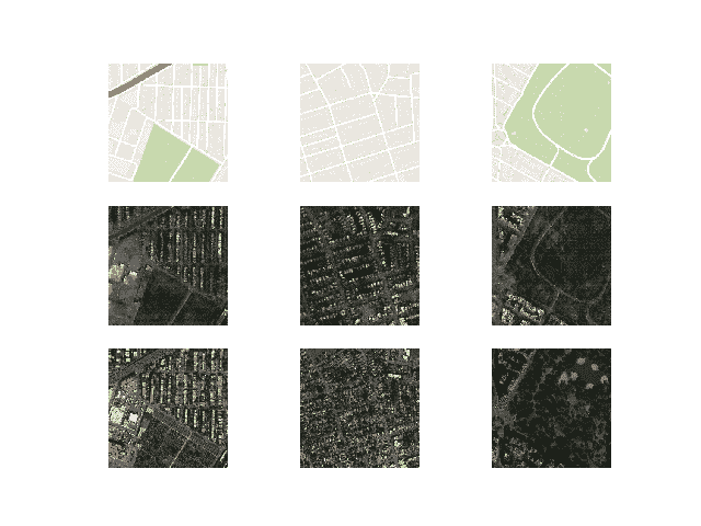
请注意下面第一个生成的图像示例(右列,中间一行),它包含比真实的谷歌地图图像更有用的细节。
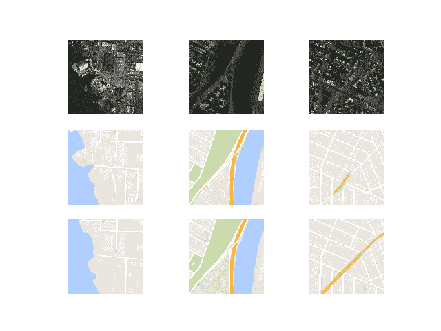
100 个训练时期后使用 Pix2Pix 绘制卫星到谷歌地图的翻译图像
现在我们已经开发并训练了 Pix2Pix 模型,我们可以探索如何以独立的方式使用它们。
如何使用 Pix2Pix 模型翻译图像
训练 Pix2Pix 模型会为每个模型生成许多保存的模型和生成的图像样本。
更多的训练时期不一定意味着更好的质量模式。因此,我们可以根据生成图像的质量选择一个模型,并使用它来执行特定的图像到图像的翻译。
在这种情况下,我们将使用运行结束时保存的模型,例如在 100 个时期或 109,600 次训练迭代之后。
一个很好的起点是加载模型,并使用它对训练数据集中的源图像进行临时翻译。
首先,我们可以加载训练数据集。我们可以使用名为 load_real_samples() 的相同函数来加载数据集,就像训练模型时使用的一样。
# load and prepare training images
def load_real_samples(filename):
	# load compressed ararys
	data = load(filename)
	# unpack arrays
	X1, X2 = data['arr_0'], data['arr_1']
	# scale from [0,255] to [-1,1]
	X1 = (X1 - 127.5) / 127.5
	X2 = (X2 - 127.5) / 127.5
	return [X1, X2]
这个函数可以如下调用:
...
# load dataset
[X1, X2] = load_real_samples('maps_256.npz')
print('Loaded', X1.shape, X2.shape)
接下来,我们可以加载保存的 Keras 模型。
...
# load model
model = load_model('model_109600.h5')
接下来,我们可以从训练数据集中选择一个随机图像对作为示例。
...
# select random example
ix = randint(0, len(X1), 1)
src_image, tar_image = X1[ix], X2[ix]
我们可以提供源卫星图像作为模型的输入,并使用它来预测谷歌地图图像。
...
# generate image from source
gen_image = model.predict(src_image)
最后,我们可以绘制源图像、生成的图像和预期的目标图像。
下面的 plot_images() 函数实现了这一点,在每个图像上方提供了一个漂亮的标题。
# plot source, generated and target images
def plot_images(src_img, gen_img, tar_img):
	images = vstack((src_img, gen_img, tar_img))
	# scale from [-1,1] to [0,1]
	images = (images + 1) / 2.0
	titles = ['Source', 'Generated', 'Expected']
	# plot images row by row
	for i in range(len(images)):
		# define subplot
		pyplot.subplot(1, 3, 1 + i)
		# turn off axis
		pyplot.axis('off')
		# plot raw pixel data
		pyplot.imshow(images[i])
		# show title
		pyplot.title(titles[i])
	pyplot.show()
这个函数可以用我们的每个源图像、生成图像和目标图像来调用。
...
# plot all three images
plot_images(src_image, gen_image, tar_image)
将所有这些结合在一起,下面列出了使用训练数据集中的一个示例执行特定图像到图像转换的完整示例。
# example of loading a pix2pix model and using it for image to image translation
from keras.models import load_model
from numpy import load
from numpy import vstack
from matplotlib import pyplot
from numpy.random import randint

# load and prepare training images
def load_real_samples(filename):
	# load compressed arrays
	data = load(filename)
	# unpack arrays
	X1, X2 = data['arr_0'], data['arr_1']
	# scale from [0,255] to [-1,1]
	X1 = (X1 - 127.5) / 127.5
	X2 = (X2 - 127.5) / 127.5
	return [X1, X2]

# plot source, generated and target images
def plot_images(src_img, gen_img, tar_img):
	images = vstack((src_img, gen_img, tar_img))
	# scale from [-1,1] to [0,1]
	images = (images + 1) / 2.0
	titles = ['Source', 'Generated', 'Expected']
	# plot images row by row
	for i in range(len(images)):
		# define subplot
		pyplot.subplot(1, 3, 1 + i)
		# turn off axis
		pyplot.axis('off')
		# plot raw pixel data
		pyplot.imshow(images[i])
		# show title
		pyplot.title(titles[i])
	pyplot.show()

# load dataset
[X1, X2] = load_real_samples('maps_256.npz')
print('Loaded', X1.shape, X2.shape)
# load model
model = load_model('model_109600.h5')
# select random example
ix = randint(0, len(X1), 1)
src_image, tar_image = X1[ix], X2[ix]
# generate image from source
gen_image = model.predict(src_image)
# plot all three images
plot_images(src_image, gen_image, tar_image)
运行该示例将从训练数据集中选择一幅随机图像,将其转换为谷歌地图,并将结果与预期图像进行比较。
注:考虑到算法或评估程序的随机性,或数值准确率的差异,您的结果可能会有所不同。考虑运行该示例几次,并比较平均结果。
在这种情况下,我们可以看到生成的图像捕捉到带有橙色和黄色以及绿色公园区域的大型道路。生成的图像并不完美,但非常接近预期图像。
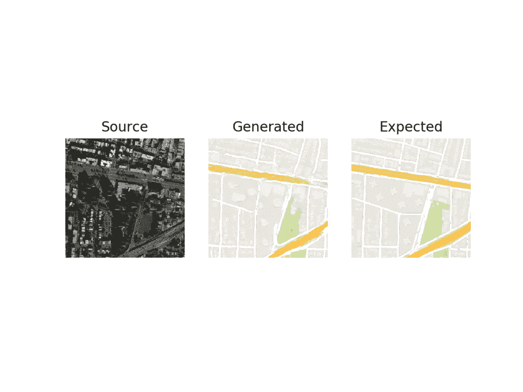
用最终的 Pix2Pix GAN 模型绘制卫星到谷歌地图的图像转换
我们可能还想使用模型来翻译给定的独立图像。
我们可以从 maps/val 下的验证数据集中选择一幅图像,并裁剪图像的卫星元素。然后可以保存并用作模型的输入。
在这种情况下,我们将使用“ maps/val/1.jpg ”。
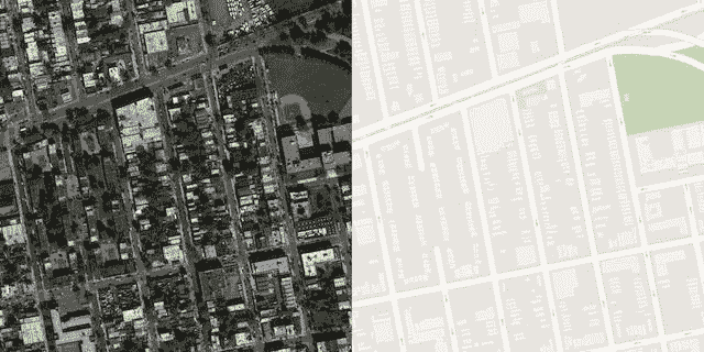
地图数据集验证部分的示例图像
我们可以使用图像程序创建该图像的卫星元素的粗略裁剪以用作输入,并将文件保存为当前工作目录中的satellite.jpg。

用作 Pix2Pix 模型输入的裁剪卫星图像示例。
我们必须将图像加载为大小为 256×256 的 NumPy 像素阵列,将像素值重新缩放到范围[-1,1],然后扩展单个图像维度以表示一个输入样本。
下面的 load_image() 函数实现了这一点,返回可以直接提供给加载的 Pix2Pix 模型的图像像素。
# load an image
def load_image(filename, size=(256,256)):
	# load image with the preferred size
	pixels = load_img(filename, target_size=size)
	# convert to numpy array
	pixels = img_to_array(pixels)
	# scale from [0,255] to [-1,1]
	pixels = (pixels - 127.5) / 127.5
	# reshape to 1 sample
	pixels = expand_dims(pixels, 0)
	return pixels
然后我们可以加载我们裁剪后的卫星图像。
...
# load source image
src_image = load_image('satellite.jpg')
print('Loaded', src_image.shape)
像以前一样,我们可以加载我们保存的 Pix2Pix 生成器模型,并生成加载图像的翻译。
...
# load model
model = load_model('model_109600.h5')
# generate image from source
gen_image = model.predict(src_image)
最后,我们可以将像素值缩放回范围[0,1]并绘制结果。
...
# scale from [-1,1] to [0,1]
gen_image = (gen_image + 1) / 2.0
# plot the image
pyplot.imshow(gen_image[0])
pyplot.axis('off')
pyplot.show()
将所有这些结合在一起,下面列出了使用单个图像文件执行临时图像转换的完整示例。
# example of loading a pix2pix model and using it for one-off image translation
from keras.models import load_model
from keras.preprocessing.image import img_to_array
from keras.preprocessing.image import load_img
from numpy import load
from numpy import expand_dims
from matplotlib import pyplot

# load an image
def load_image(filename, size=(256,256)):
	# load image with the preferred size
	pixels = load_img(filename, target_size=size)
	# convert to numpy array
	pixels = img_to_array(pixels)
	# scale from [0,255] to [-1,1]
	pixels = (pixels - 127.5) / 127.5
	# reshape to 1 sample
	pixels = expand_dims(pixels, 0)
	return pixels

# load source image
src_image = load_image('satellite.jpg')
print('Loaded', src_image.shape)
# load model
model = load_model('model_109600.h5')
# generate image from source
gen_image = model.predict(src_image)
# scale from [-1,1] to [0,1]
gen_image = (gen_image + 1) / 2.0
# plot the image
pyplot.imshow(gen_image[0])
pyplot.axis('off')
pyplot.show()
运行该示例从文件加载图像,创建图像的翻译,并绘制结果。
生成的图像似乎是源图像的合理翻译。
街道看起来不是直线,建筑的细节有点欠缺。也许通过进一步的训练或选择不同的模型,可以生成更高质量的图像。
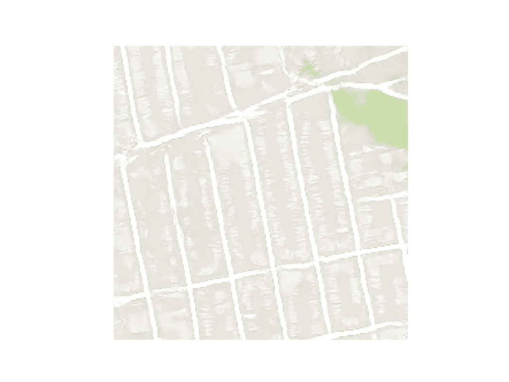
最终 Pix2Pix GAN 模型转换为谷歌地图的卫星图像图
如何将谷歌地图翻译成卫星图像
既然我们已经熟悉了如何开发和使用 Pix2Pix 模型将卫星图像转换成谷歌地图,我们也可以探索相反的情况。
也就是说,我们可以开发一个 Pix2Pix 模型,将谷歌地图图像转换成可信的卫星图像。这需要模型发明或产生似是而非的建筑、道路、公园等等。
我们可以使用相同的代码来训练模型,只有一点点不同。我们可以改变 load_real_samples() 函数返回的数据集的顺序;例如:
# load and prepare training images
def load_real_samples(filename):
	# load compressed arrays
	data = load(filename)
	# unpack arrays
	X1, X2 = data['arr_0'], data['arr_1']
	# scale from [0,255] to [-1,1]
	X1 = (X1 - 127.5) / 127.5
	X2 = (X2 - 127.5) / 127.5
	# return in reverse order
	return [X2, X1]
注:X1 和 X2 的顺序颠倒。
这意味着该模型将以谷歌地图图像为输入,并学习生成卫星图像。
像以前一样运行示例。
注:考虑到算法或评估程序的随机性,或数值准确率的差异,您的结果可能会有所不同。考虑运行该示例几次,并比较平均结果。
和以前一样,在每次训练迭代中都会报告模型的丢失。如果鉴别器的损耗变为零并在那里停留很长时间,考虑重新开始训练,因为这是训练失败的一个例子。
>1, d1[0.442] d2[0.650] g[49.790]
>2, d1[0.317] d2[0.478] g[56.476]
>3, d1[0.376] d2[0.450] g[48.114]
>4, d1[0.396] d2[0.406] g[62.903]
>5, d1[0.496] d2[0.460] g[40.650]
...
>109596, d1[0.311] d2[0.057] g[25.376]
>109597, d1[0.028] d2[0.070] g[16.618]
>109598, d1[0.007] d2[0.208] g[18.139]
>109599, d1[0.358] d2[0.076] g[22.494]
>109600, d1[0.279] d2[0.049] g[9.941]
>Saved: plot_109600.png and model_109600.h5
很难判断生成的卫星图像的质量,尽管如此,看似可信的图像仅在 10 个时代后就生成了。
使用 Pix2Pix 绘制 10 个训练时期后的谷歌地图到卫星翻译图像
像以前一样,图像质量将会提高,并且在训练过程中会继续变化。最终模型可以基于生成的图像质量来选择,而不是基于总的训练时期。
该模型在生成合理的水、公园、道路等方面似乎没有什么困难。

使用 Pix2Pix 绘制 90 后训练时期的谷歌地图到卫星翻译图像
扩展ˌ扩张
本节列出了一些您可能希望探索的扩展教程的想法。
- 独立卫星。开发一个将独立的谷歌地图图像转换为卫星图像的例子,就像我们对卫星到谷歌地图图像所做的那样。
- 新形象。找到一个全新位置的卫星图像,并将其转换为谷歌地图,然后将结果与谷歌地图中的实际图像进行比较。
- 更多训练。继续为另一个 100 个时期训练模型,并评估额外的训练是否导致图像质量的进一步提高。
- 图像扩充。按照 Pix2Pix 论文中的描述,在训练过程中使用一些小的图像扩充,并评估它是否会产生更好质量的生成图像。
如果你探索这些扩展,我很想知道。
在下面的评论中发表你的发现。
进一步阅读
如果您想更深入地了解这个主题,本节将提供更多资源。
正式的
- 条件对抗网络下的图像到图像转换,2016。
- 带条件对抗网的图像到图像转换,主页。
- 带条件对抗网的图像到图像转换,GitHub 。
- pytorch-cyclelegan-and-pix 2 pix,GitHub 。
- 互动影像转影像演示,2017 年。
- Pix2Pix 数据集
应用程序接口
摘要
在本教程中,您发现了如何为图像到图像的翻译开发一个 Pix2Pix 生成式对抗网络。
具体来说,您了解到:
- 如何将卫星图像加载并准备到谷歌地图图像到图像转换数据集。
- 如何开发一个 Pix2Pix 模型,用于将卫星照片翻译成谷歌地图图像。
- 如何使用最终的 Pix2Pix 生成器模型来翻译临时卫星图像。
你有什么问题吗?
在下面的评论中提问,我会尽力回答。
如何用 Keras 从零开始开发辅助分类器 GAN(AC-GAN)
最后更新于 2021 年 1 月 18 日
生成对抗网络是一种用于训练生成模型的体系结构,例如用于生成图像的深度卷积神经网络。
条件生成对抗网络,简称 cGAN,是一种 GAN,涉及到通过生成器模型有条件地生成图像。图像生成可以以类标签为条件(如果可用),允许有针对性地生成给定类型的图像。
辅助分类器 GAN,简称 AC-GAN,是条件 GAN 的扩展,它改变鉴别器来预测给定图像的类别标签,而不是接收它作为输入。它具有稳定训练过程的效果,并允许生成大的高质量图像,同时学习独立于类别标签的潜在空间中的表示。
在本教程中,您将发现如何开发一个辅助分类器生成对抗网络来生成服装照片。
完成本教程后,您将知道:
- 辅助分类器 GAN 是一种条件 GAN,它要求鉴别器预测给定图像的类别标签。
- 如何开发交流 GAN 的发生器、鉴别器和复合模型。
- 如何训练、评估和使用 AC-GAN 从时尚 MNIST 数据集生成服装照片。
用我的新书Python 生成对抗网络启动你的项目,包括分步教程和所有示例的 Python 源代码文件。
我们开始吧。
- 2021 年 1 月更新:更新所以层冻结用批量定额。
如何用 Keras 从零开始开发辅助分类器 GAN (AC-GAN)图片由 ebbe ostebo 提供,版权所有。
教程概述
本教程分为五个部分;它们是:
- 辅助分类器生成对抗网络
- 时尚-MNIST 服装照片数据集
- 如何定义交流 GAN 模型
- 如何为时尚 MNIST 开发交流 GAN
- 如何用人工智能生成服装项目
辅助分类器生成对抗网络
生成对抗网络是一种用于训练生成模型的体系结构,通常是用于生成图像的深度卷积神经网络。
该架构由一个生成器模型和一个鉴别器组成,生成器模型从潜在空间中获取随机点作为输入并生成图像,鉴别器用于将图像分类为真实(来自数据集)或虚假(生成)。然后在零和游戏中同时训练两个模型。
有条件的 GAN,简称 CGAN 或 cGAN,是 GAN 架构的扩展,为潜在空间增加了结构。改变 GAN 模型的训练,使得生成器被提供潜在空间中的点和类别标签作为输入,并且尝试为该类别生成图像。鉴别器提供有图像和类别标签,并且必须像以前一样分类图像是真的还是假的。
添加类作为输入使得图像生成过程和图像分类过程以类标签为条件,因此得名。其效果是更稳定的训练过程和生成的生成器模型,该生成器模型可用于生成给定特定类型的图像,例如用于类别标签。
辅助分类器 GAN,简称 AC-GAN,是基于 CGAN 扩展的 GAN 体系结构的进一步扩展。它是由 Augustus Odena 等人从 Google Brain 在 2016 年发表的论文《使用辅助分类器 GANs 的条件图像合成》中引入的
与有条件的 GAN 一样,AC-GAN 中的生成器模型被提供有潜在空间中的点和作为输入的类别标签,例如图像生成过程是有条件的。
主要区别在于鉴别器模型,它只提供图像作为输入,不像条件 GAN 提供图像和类标签作为输入。然后,鉴别器模型必须像以前一样预测给定图像是真的还是假的,并且还必须预测图像的类别标签。
……模型[…]是有类条件的,但带有一个负责重构类标签的辅助解码器。
——辅助分类器条件图像合成 GANs ,2016。
该体系结构以这样的方式描述,即鉴别器和辅助分类器可以被认为是共享模型权重的独立模型。在实践中,鉴别器和辅助分类器可以实现为具有两个输出的单个神经网络模型。
第一个输出是通过 sigmoid 激活函数的单个概率,表示输入图像的“真实度”,并使用二进制交叉熵进行优化,就像正常的 GAN 鉴别器模型一样。
第二输出是图像经由 softmax 激活函数属于每个类别的概率,像任何给定的多类别分类神经网络模型一样,并且使用分类交叉熵进行优化。
总结一下:
发电机型号:
- 输入:来自潜在空间的随机点,以及类别标签。
- 输出:生成的图像。
鉴别器模型:
- 输入:图像。
- 输出:提供的图像真实的概率,图像属于每个已知类别的概率。
下图总结了一系列条件 GAN 的输入和输出,包括交流 GAN,提供了一些差异的背景。
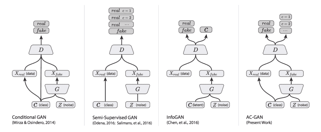
条件 GAN、半监督 GAN、信息 GAN 和交流 GAN 之间的差异总结。
摘自:辅助分类器 GANs 条件图像合成版。
鉴别器寻求最大化正确分类真实和虚假图像的概率,并正确预测真实或虚假图像(例如,真实图像+虚假图像)的类别标签。生成器寻求最小化鉴别器鉴别真实和伪造图像的能力,同时也最大化鉴别器预测真实和伪造图像的类别标签的能力(例如 LC–LS)。
目标函数有两个部分:正确源的对数似然性 LS 和正确类的对数似然性 LC。[……]D 被训练为最大化最小二乘+最小二乘,而 G 被训练为最大化最小二乘。
——辅助分类器条件图像合成 GANs ,2016。
生成的生成器学习独立于类标签的潜在空间表示,不像条件 GAN。
AC-GANs 学习独立于类标签的 z 的表示。
——辅助分类器条件图像合成 GANs ,2016。
以这种方式改变条件 GAN 的效果是更稳定的训练过程和模型生成比以前可能的更大尺寸(例如 128×128 像素)的更高质量图像的能力。
……我们证明,向 GAN 潜在空间添加更多结构以及专门的成本函数,可以获得更高质量的样本。[……]重要的是,我们从数量上证明了我们的高分辨率样本不仅仅是低分辨率样本的简单重置。
——辅助分类器条件图像合成 GANs ,2016。
时尚-MNIST 服装照片数据集
时尚-MNIST 数据集被提议作为 MNIST 手写数字数据集的更具挑战性的替换数据集。
它是一个数据集,由 60,000 个 28×28 像素的小正方形灰度图像组成,包括 10 种服装,如鞋子、t 恤、连衣裙等。
Keras 通过 fashion_mnist.load_dataset()函数提供对时尚 MNIST 数据集的访问。它返回两个元组,一个包含标准训练数据集的输入和输出元素,另一个包含标准测试数据集的输入和输出元素。
下面的示例加载数据集并总结加载数据集的形状。
注意:第一次加载数据集时,Keras 会自动下载图片的压缩版本,保存在的主目录下~/。keras/数据集/ 。下载速度很快,因为压缩形式的数据集只有大约 25 兆字节。
# example of loading the fashion_mnist dataset
from keras.datasets.fashion_mnist import load_data
# load the images into memory
(trainX, trainy), (testX, testy) = load_data()
# summarize the shape of the dataset
print('Train', trainX.shape, trainy.shape)
print('Test', testX.shape, testy.shape)
运行该示例将加载数据集,并打印训练的输入和输出组件的形状,以及测试图像的分割。
我们可以看到训练集中有 60K 个例子,测试集中有 10K,每个图像都是 28 乘 28 像素的正方形。
Train (60000, 28, 28) (60000,)
Test (10000, 28, 28) (10000,)
图像是黑色背景(像素值为 0)的灰度图像,衣服是白色的(像素值接近 255)。这意味着如果图像被绘制出来,它们大部分是黑色的,中间有一件白色的衣服。
我们可以使用带有 imshow()函数的 matplotlib 库绘制训练数据集中的一些图像,并通过“ cmap ”参数将颜色映射指定为“灰色,以正确显示像素值。
# plot raw pixel data
pyplot.imshow(trainX[i], cmap='gray')
或者,当我们颠倒颜色,将背景画成白色,将服装画成黑色时,图像更容易查看。
它们更容易观看,因为大部分图像现在是白色的,而感兴趣的区域是黑色的。这可以通过使用反向灰度色图来实现,如下所示:
# plot raw pixel data
pyplot.imshow(trainX[i], cmap='gray_r')
以下示例将训练数据集中的前 100 幅图像绘制成 10 乘 10 的正方形。
# example of loading the fashion_mnist dataset
from keras.datasets.fashion_mnist import load_data
from matplotlib import pyplot
# load the images into memory
(trainX, trainy), (testX, testy) = load_data()
# plot images from the training dataset
for i in range(100):
	# define subplot
	pyplot.subplot(10, 10, 1 + i)
	# turn off axis
	pyplot.axis('off')
	# plot raw pixel data
	pyplot.imshow(trainX[i], cmap='gray_r')
pyplot.show()
运行该示例会创建一个图形,其中包含 100 幅来自 MNIST 训练数据集的图像,排列成 10×10 的正方形。
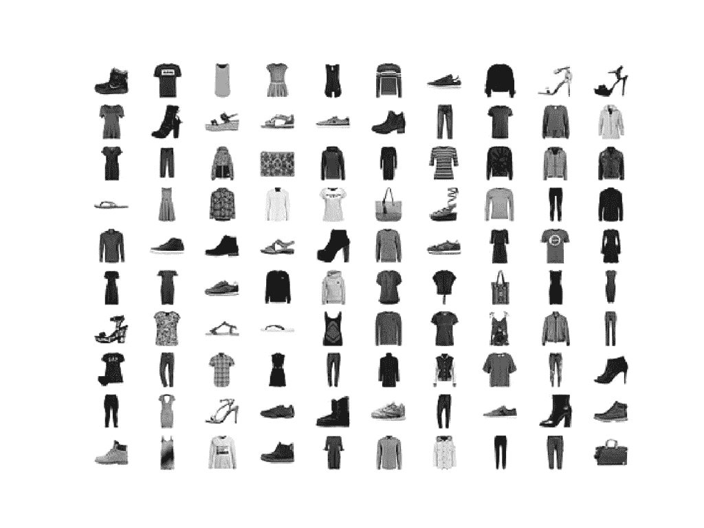
时尚 MNIST 数据集中前 100 件服装的图表。
我们将使用训练数据集中的图像作为训练生成对抗网络的基础。
具体来说,生成器模型将学习如何生成新的似是而非的服装项目,使用鉴别器来尝试区分来自时尚 MNIST 训练数据集的真实图像和生成器模型输出的新图像,并预测每个图像的类别标签。
这是一个相对简单的问题,不需要复杂的生成器或鉴别器模型,尽管它确实需要生成灰度输出图像。
如何定义交流 GAN 模型
在本节中,我们将开发交流 GAN 的发生器、鉴别器和复合模型。
交流-GAN 论文的附录提供了发电机和鉴频器配置的建议,我们将用作灵感。下表总结了本文中对 CIFAR-10 数据集的建议。

交流-GAN 发电机和鉴别器型号配置建议。
取自:使用辅助分类器 GANs 的条件图像合成。
交流-GAN 鉴别器模型
让我们从鉴别器模型开始。
鉴别器模型必须将图像作为输入,并且预测图像的真实度的概率和图像属于每个给定类别的概率。
输入图像的形状为 28x28x1,在时尚 MNIST 数据集中有 10 个服装类别。
该模型可以按照 DCGAN 架构进行定义。也就是说,使用高斯权重初始化、批处理归一化、LeakyReLU、Dropout 和 2×2 步长进行下采样,而不是合并层。
例如,下面是使用 Keras 函数 API 定义的鉴别器模型的主体。
...
# weight initialization
init = RandomNormal(stddev=0.02)
# image input
in_image = Input(shape=in_shape)
# downsample to 14x14
fe = Conv2D(32, (3,3), strides=(2,2), padding='same', kernel_initializer=init)(in_image)
fe = LeakyReLU(alpha=0.2)(fe)
fe = Dropout(0.5)(fe)
# normal
fe = Conv2D(64, (3,3), padding='same', kernel_initializer=init)(fe)
fe = BatchNormalization()(fe)
fe = LeakyReLU(alpha=0.2)(fe)
fe = Dropout(0.5)(fe)
# downsample to 7x7
fe = Conv2D(128, (3,3), strides=(2,2), padding='same', kernel_initializer=init)(fe)
fe = BatchNormalization()(fe)
fe = LeakyReLU(alpha=0.2)(fe)
fe = Dropout(0.5)(fe)
# normal
fe = Conv2D(256, (3,3), padding='same', kernel_initializer=init)(fe)
fe = BatchNormalization()(fe)
fe = LeakyReLU(alpha=0.2)(fe)
fe = Dropout(0.5)(fe)
# flatten feature maps
fe = Flatten()(fe)
...
主要区别在于模型有两个输出层。
第一个是单个节点,具有 sigmoid 激活,用于预测图像的真实性。
...
# real/fake output
out1 = Dense(1, activation='sigmoid')(fe)
第二种是多个节点,每个类一个,使用 softmax 激活函数来预测给定图像的类标签。
...
# class label output
out2 = Dense(n_classes, activation='softmax')(fe)
然后,我们可以用一个输入和两个输出来构建图像。
...
# define model
model = Model(in_image, [out1, out2])
该模型必须用两个损失函数训练,第一输出层的二元交叉熵和第二输出层的分类交叉熵损失。
我们可以直接比较整数类标签,而不是像通常那样将类标签的一个热编码与第二个输出层进行比较。我们可以使用稀疏分类交叉熵损失函数自动实现这一点。这将具有分类交叉熵的相同效果,但是避免了必须手动对目标标签进行一次热编码的步骤。
在编译模型时,我们可以通过将函数名列表指定为字符串来通知 Keras 对两个输出层使用两个不同的损失函数;例如:
loss=['binary_crossentropy', 'sparse_categorical_crossentropy']
该模型使用随机梯度下降的 Adam 版本进行拟合,学习率小,动量适中,这是 DCGANs 推荐的。
...
# compile model
opt = Adam(lr=0.0002, beta_1=0.5)
model.compile(loss=['binary_crossentropy', 'sparse_categorical_crossentropy'], optimizer=opt)
将这些联系在一起,define_discriminator()函数将为 AC-GAN 定义和编译鉴别器模型。
输入图像的形状和类的数量是参数化的,并使用默认值进行设置,允许它们在将来为您自己的项目轻松更改。
# define the standalone discriminator model
def define_discriminator(in_shape=(28,28,1), n_classes=10):
	# weight initialization
	init = RandomNormal(stddev=0.02)
	# image input
	in_image = Input(shape=in_shape)
	# downsample to 14x14
	fe = Conv2D(32, (3,3), strides=(2,2), padding='same', kernel_initializer=init)(in_image)
	fe = LeakyReLU(alpha=0.2)(fe)
	fe = Dropout(0.5)(fe)
	# normal
	fe = Conv2D(64, (3,3), padding='same', kernel_initializer=init)(fe)
	fe = BatchNormalization()(fe)
	fe = LeakyReLU(alpha=0.2)(fe)
	fe = Dropout(0.5)(fe)
	# downsample to 7x7
	fe = Conv2D(128, (3,3), strides=(2,2), padding='same', kernel_initializer=init)(fe)
	fe = BatchNormalization()(fe)
	fe = LeakyReLU(alpha=0.2)(fe)
	fe = Dropout(0.5)(fe)
	# normal
	fe = Conv2D(256, (3,3), padding='same', kernel_initializer=init)(fe)
	fe = BatchNormalization()(fe)
	fe = LeakyReLU(alpha=0.2)(fe)
	fe = Dropout(0.5)(fe)
	# flatten feature maps
	fe = Flatten()(fe)
	# real/fake output
	out1 = Dense(1, activation='sigmoid')(fe)
	# class label output
	out2 = Dense(n_classes, activation='softmax')(fe)
	# define model
	model = Model(in_image, [out1, out2])
	# compile model
	opt = Adam(lr=0.0002, beta_1=0.5)
	model.compile(loss=['binary_crossentropy', 'sparse_categorical_crossentropy'], optimizer=opt)
	return model
我们可以定义和总结这个模型。
下面列出了完整的示例。
# example of defining the discriminator model
from keras.models import Model
from keras.layers import Input
from keras.layers import Dense
from keras.layers import Conv2D
from keras.layers import LeakyReLU
from keras.layers import Dropout
from keras.layers import Flatten
from keras.layers import BatchNormalization
from keras.initializers import RandomNormal
from keras.optimizers import Adam
from keras.utils.vis_utils import plot_model

# define the standalone discriminator model
def define_discriminator(in_shape=(28,28,1), n_classes=10):
	# weight initialization
	init = RandomNormal(stddev=0.02)
	# image input
	in_image = Input(shape=in_shape)
	# downsample to 14x14
	fe = Conv2D(32, (3,3), strides=(2,2), padding='same', kernel_initializer=init)(in_image)
	fe = LeakyReLU(alpha=0.2)(fe)
	fe = Dropout(0.5)(fe)
	# normal
	fe = Conv2D(64, (3,3), padding='same', kernel_initializer=init)(fe)
	fe = BatchNormalization()(fe)
	fe = LeakyReLU(alpha=0.2)(fe)
	fe = Dropout(0.5)(fe)
	# downsample to 7x7
	fe = Conv2D(128, (3,3), strides=(2,2), padding='same', kernel_initializer=init)(fe)
	fe = BatchNormalization()(fe)
	fe = LeakyReLU(alpha=0.2)(fe)
	fe = Dropout(0.5)(fe)
	# normal
	fe = Conv2D(256, (3,3), padding='same', kernel_initializer=init)(fe)
	fe = BatchNormalization()(fe)
	fe = LeakyReLU(alpha=0.2)(fe)
	fe = Dropout(0.5)(fe)
	# flatten feature maps
	fe = Flatten()(fe)
	# real/fake output
	out1 = Dense(1, activation='sigmoid')(fe)
	# class label output
	out2 = Dense(n_classes, activation='softmax')(fe)
	# define model
	model = Model(in_image, [out1, out2])
	# compile model
	opt = Adam(lr=0.0002, beta_1=0.5)
	model.compile(loss=['binary_crossentropy', 'sparse_categorical_crossentropy'], optimizer=opt)
	return model

# define the discriminator model
model = define_discriminator()
# summarize the model
model.summary()
# plot the model
plot_model(model, to_file='discriminator_plot.png', show_shapes=True, show_layer_names=True)
运行示例首先打印模型的摘要。
这确认了输入图像和两个输出层的预期形状,尽管线性组织确实使两个独立的输出层清晰。
__________________________________________________________________________________________________
Layer (type)                    Output Shape         Param #     Connected to
==================================================================================================
input_1 (InputLayer)            (None, 28, 28, 1)    0
__________________________________________________________________________________________________
conv2d_1 (Conv2D)               (None, 14, 14, 32)   320         input_1[0][0]
__________________________________________________________________________________________________
leaky_re_lu_1 (LeakyReLU)       (None, 14, 14, 32)   0           conv2d_1[0][0]
__________________________________________________________________________________________________
dropout_1 (Dropout)             (None, 14, 14, 32)   0           leaky_re_lu_1[0][0]
__________________________________________________________________________________________________
conv2d_2 (Conv2D)               (None, 14, 14, 64)   18496       dropout_1[0][0]
__________________________________________________________________________________________________
batch_normalization_1 (BatchNor (None, 14, 14, 64)   256         conv2d_2[0][0]
__________________________________________________________________________________________________
leaky_re_lu_2 (LeakyReLU)       (None, 14, 14, 64)   0           batch_normalization_1[0][0]
__________________________________________________________________________________________________
dropout_2 (Dropout)             (None, 14, 14, 64)   0           leaky_re_lu_2[0][0]
__________________________________________________________________________________________________
conv2d_3 (Conv2D)               (None, 7, 7, 128)    73856       dropout_2[0][0]
__________________________________________________________________________________________________
batch_normalization_2 (BatchNor (None, 7, 7, 128)    512         conv2d_3[0][0]
__________________________________________________________________________________________________
leaky_re_lu_3 (LeakyReLU)       (None, 7, 7, 128)    0           batch_normalization_2[0][0]
__________________________________________________________________________________________________
dropout_3 (Dropout)             (None, 7, 7, 128)    0           leaky_re_lu_3[0][0]
__________________________________________________________________________________________________
conv2d_4 (Conv2D)               (None, 7, 7, 256)    295168      dropout_3[0][0]
__________________________________________________________________________________________________
batch_normalization_3 (BatchNor (None, 7, 7, 256)    1024        conv2d_4[0][0]
__________________________________________________________________________________________________
leaky_re_lu_4 (LeakyReLU)       (None, 7, 7, 256)    0           batch_normalization_3[0][0]
__________________________________________________________________________________________________
dropout_4 (Dropout)             (None, 7, 7, 256)    0           leaky_re_lu_4[0][0]
__________________________________________________________________________________________________
flatten_1 (Flatten)             (None, 12544)        0           dropout_4[0][0]
__________________________________________________________________________________________________
dense_1 (Dense)                 (None, 1)            12545       flatten_1[0][0]
__________________________________________________________________________________________________
dense_2 (Dense)                 (None, 10)           125450      flatten_1[0][0]
==================================================================================================
Total params: 527,627
Trainable params: 526,731
Non-trainable params: 896
__________________________________________________________________________________________________
还会创建一个模型图,显示输入图像的线性处理和两个清晰的输出层。

辅助分类器 GAN 的鉴别器模型图
既然我们已经定义了交流-GAN 鉴别器模型,我们就可以开发发电机模型了。
交流 GAN 发电机模型
生成器模型必须从潜在空间中取一个随机点作为输入,并加上类标签,然后输出一个形状为 28x28x1 的生成灰度图像。
AC-GAN 论文描述了 AC-GAN 生成器模型,该模型采用矢量输入,该矢量输入是潜在空间中的点(100 维)和一个热编码类标签(10 维)的级联,该标签为 110 维。
一种已经被证明有效并且现在被普遍推荐的替代方法是在生成器模型的早期将类标签解释为附加的通道或特征图。
这可以通过使用具有任意维数(例如 50)的学习嵌入来实现,其输出可以由具有线性激活的完全连接的层来解释,从而产生一个额外的 7×7 特征图。
...
# label input
in_label = Input(shape=(1,))
# embedding for categorical input
li = Embedding(n_classes, 50)(in_label)
# linear multiplication
n_nodes = 7 * 7
li = Dense(n_nodes, kernel_initializer=init)(li)
# reshape to additional channel
li = Reshape((7, 7, 1))(li)
潜在空间中的点可以由具有足够激活的完全连接的层来解释,以创建多个 7×7 特征图,在本例中为 384,并为我们的输出图像的低分辨率版本提供基础。
类别标签的 7×7 单要素地图解释然后可以按通道连接,从而产生 385 个要素地图。
...
# image generator input
in_lat = Input(shape=(latent_dim,))
# foundation for 7x7 image
n_nodes = 384 * 7 * 7
gen = Dense(n_nodes, kernel_initializer=init)(in_lat)
gen = Activation('relu')(gen)
gen = Reshape((7, 7, 384))(gen)
# merge image gen and label input
merge = Concatenate()([gen, li])
然后,这些特征图可以经历两个转置卷积层的过程,以将 7×7 特征图首先上采样到 14×14 像素,然后最后上采样到 28×28 特征,随着每个上缩放步骤,特征图的面积翻了两番。
发生器的输出是一个单一的特征图或灰度图像,形状为 28×28,像素值在范围[-1,1]内,给定 tanh 激活函数的选择。我们使用 ReLU 激活来升级层,而不是 AC-GAN 论文中给出的 LeakyReLU。
# upsample to 14x14
gen = Conv2DTranspose(192, (5,5), strides=(2,2), padding='same', kernel_initializer=init)(merge)
gen = BatchNormalization()(gen)
gen = Activation('relu')(gen)
# upsample to 28x28
gen = Conv2DTranspose(1, (5,5), strides=(2,2), padding='same', kernel_initializer=init)(gen)
out_layer = Activation('tanh')(gen)
我们可以将所有这些联系在一起,并结合到下面定义的 define_generator()函数中,该函数将创建并返回交流-GAN 的发电机模型。
模型不是直接训练的,所以故意不编译;相反,它是通过鉴别器模型训练的。
# define the standalone generator model
def define_generator(latent_dim, n_classes=10):
	# weight initialization
	init = RandomNormal(stddev=0.02)
	# label input
	in_label = Input(shape=(1,))
	# embedding for categorical input
	li = Embedding(n_classes, 50)(in_label)
	# linear multiplication
	n_nodes = 7 * 7
	li = Dense(n_nodes, kernel_initializer=init)(li)
	# reshape to additional channel
	li = Reshape((7, 7, 1))(li)
	# image generator input
	in_lat = Input(shape=(latent_dim,))
	# foundation for 7x7 image
	n_nodes = 384 * 7 * 7
	gen = Dense(n_nodes, kernel_initializer=init)(in_lat)
	gen = Activation('relu')(gen)
	gen = Reshape((7, 7, 384))(gen)
	# merge image gen and label input
	merge = Concatenate()([gen, li])
	# upsample to 14x14
	gen = Conv2DTranspose(192, (5,5), strides=(2,2), padding='same', kernel_initializer=init)(merge)
	gen = BatchNormalization()(gen)
	gen = Activation('relu')(gen)
	# upsample to 28x28
	gen = Conv2DTranspose(1, (5,5), strides=(2,2), padding='same', kernel_initializer=init)(gen)
	out_layer = Activation('tanh')(gen)
	# define model
	model = Model([in_lat, in_label], out_layer)
	return model
我们可以创建这个模型,并总结和绘制它的结构。
下面列出了完整的示例。
# example of defining the generator model
from keras.models import Model
from keras.layers import Input
from keras.layers import Dense
from keras.layers import Reshape
from keras.layers import Conv2DTranspose
from keras.layers import Embedding
from keras.layers import Concatenate
from keras.layers import Activation
from keras.layers import BatchNormalization
from keras.initializers import RandomNormal
from keras.utils.vis_utils import plot_model

# define the standalone generator model
def define_generator(latent_dim, n_classes=10):
	# weight initialization
	init = RandomNormal(stddev=0.02)
	# label input
	in_label = Input(shape=(1,))
	# embedding for categorical input
	li = Embedding(n_classes, 50)(in_label)
	# linear multiplication
	n_nodes = 7 * 7
	li = Dense(n_nodes, kernel_initializer=init)(li)
	# reshape to additional channel
	li = Reshape((7, 7, 1))(li)
	# image generator input
	in_lat = Input(shape=(latent_dim,))
	# foundation for 7x7 image
	n_nodes = 384 * 7 * 7
	gen = Dense(n_nodes, kernel_initializer=init)(in_lat)
	gen = Activation('relu')(gen)
	gen = Reshape((7, 7, 384))(gen)
	# merge image gen and label input
	merge = Concatenate()([gen, li])
	# upsample to 14x14
	gen = Conv2DTranspose(192, (5,5), strides=(2,2), padding='same', kernel_initializer=init)(merge)
	gen = BatchNormalization()(gen)
	gen = Activation('relu')(gen)
	# upsample to 28x28
	gen = Conv2DTranspose(1, (5,5), strides=(2,2), padding='same', kernel_initializer=init)(gen)
	out_layer = Activation('tanh')(gen)
	# define model
	model = Model([in_lat, in_label], out_layer)
	return model

# define the size of the latent space
latent_dim = 100
# define the generator model
model = define_generator(latent_dim)
# summarize the model
model.summary()
# plot the model
plot_model(model, to_file='generator_plot.png', show_shapes=True, show_layer_names=True)
运行该示例首先打印模型中层及其输出形状的摘要。
我们可以确认潜在维度输入是 100 个维度,类标签输入是单个整数。我们还可以确认嵌入类标签的的输出被正确连接为附加通道,从而在转置卷积层之前产生 385 个 7×7 特征映射。
总结还确认了单个灰度 28×28 图像的预期输出形状。
__________________________________________________________________________________________________
Layer (type)                    Output Shape         Param #     Connected to
==================================================================================================
input_2 (InputLayer)            (None, 100)          0
__________________________________________________________________________________________________
input_1 (InputLayer)            (None, 1)            0
__________________________________________________________________________________________________
dense_2 (Dense)                 (None, 18816)        1900416     input_2[0][0]
__________________________________________________________________________________________________
embedding_1 (Embedding)         (None, 1, 50)        500         input_1[0][0]
__________________________________________________________________________________________________
activation_1 (Activation)       (None, 18816)        0           dense_2[0][0]
__________________________________________________________________________________________________
dense_1 (Dense)                 (None, 1, 49)        2499        embedding_1[0][0]
__________________________________________________________________________________________________
reshape_2 (Reshape)             (None, 7, 7, 384)    0           activation_1[0][0]
__________________________________________________________________________________________________
reshape_1 (Reshape)             (None, 7, 7, 1)      0           dense_1[0][0]
__________________________________________________________________________________________________
concatenate_1 (Concatenate)     (None, 7, 7, 385)    0           reshape_2[0][0]
                                                                 reshape_1[0][0]
__________________________________________________________________________________________________
conv2d_transpose_1 (Conv2DTrans (None, 14, 14, 192)  1848192     concatenate_1[0][0]
__________________________________________________________________________________________________
batch_normalization_1 (BatchNor (None, 14, 14, 192)  768         conv2d_transpose_1[0][0]
__________________________________________________________________________________________________
activation_2 (Activation)       (None, 14, 14, 192)  0           batch_normalization_1[0][0]
__________________________________________________________________________________________________
conv2d_transpose_2 (Conv2DTrans (None, 28, 28, 1)    4801        activation_2[0][0]
__________________________________________________________________________________________________
activation_3 (Activation)       (None, 28, 28, 1)    0           conv2d_transpose_2[0][0]
==================================================================================================
Total params: 3,757,176
Trainable params: 3,756,792
Non-trainable params: 384
__________________________________________________________________________________________________
还会创建网络图,总结每层的输入和输出形状。
该图确认了网络的两个输入以及输入的正确连接。
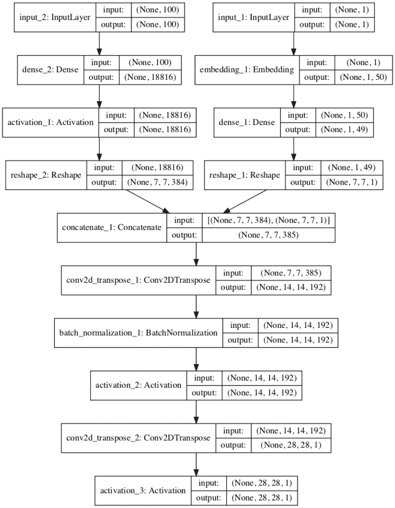
辅助分类器 GAN 发生器模型图
现在我们已经定义了生成器模型,我们可以展示它可能是如何适合的。
交流-GAN 复合模型
发电机型号不直接更新;相反,它通过鉴别器模型进行更新。
这可以通过创建一个复合模型来实现,该模型将生成器模型堆叠在鉴别器模型之上。
这个复合模型的输入是生成器模型的输入,即来自潜在空间的随机点和类标签。生成器模型直接连接到鉴别器模型,鉴别器模型直接将生成的图像作为输入。最后,鉴别器模型预测生成的图像和类别标签的真实性。因此,使用两个损失函数优化复合模型,鉴别器模型的每个输出对应一个损失函数。
鉴别器模型以独立的方式使用真实和虚假的例子进行更新,我们将在下一节回顾如何做到这一点。因此,我们不希望在更新(训练)复合模型时更新鉴别器模型;我们只想使用这个复合模型来更新生成器模型的权重。
这可以通过在编译复合模型之前将鉴别器的层设置为不可训练来实现。这仅在复合模型查看或使用时对层权重有影响,并防止它们在复合模型更新时被更新。
下面的 define_gan() 函数实现了这一点,将已经定义的生成器和鉴别器模型作为输入,并定义了一个新的复合模型,该模型只能用于更新生成器模型。
# define the combined generator and discriminator model, for updating the generator
def define_gan(g_model, d_model):
	# make weights in the discriminator not trainable
	for layer in d_model.layers:
		if not isinstance(layer, BatchNormalization):
			layer.trainable = False
	# connect the outputs of the generator to the inputs of the discriminator
	gan_output = d_model(g_model.output)
	# define gan model as taking noise and label and outputting real/fake and label outputs
	model = Model(g_model.input, gan_output)
	# compile model
	opt = Adam(lr=0.0002, beta_1=0.5)
	model.compile(loss=['binary_crossentropy', 'sparse_categorical_crossentropy'], optimizer=opt)
	return model
现在我们已经定义了 AC-GAN 中使用的模型,我们可以将它们放在时尚-MNIST 数据集上。
如何为时尚 MNIST 开发交流 GAN
第一步是加载和准备时尚 MNIST 数据集。
我们只需要训练数据集中的图像。图像是黑白的,因此我们必须增加一个额外的通道维度来将它们转换成三维的,正如我们模型的卷积层所预期的那样。最后,像素值必须缩放到范围[-1,1]以匹配生成器模型的输出。
下面的 load_real_samples() 函数实现了这一点,返回加载并缩放的时尚 MNIST 训练数据集,准备建模。
# load images
def load_real_samples():
	# load dataset
	(trainX, trainy), (_, _) = load_data()
	# expand to 3d, e.g. add channels
	X = expand_dims(trainX, axis=-1)
	# convert from ints to floats
	X = X.astype('float32')
	# scale from [0,255] to [-1,1]
	X = (X - 127.5) / 127.5
	print(X.shape, trainy.shape)
	return [X, trainy]
我们将需要数据集的一批(或半批)真实图像来更新 GAN 模型。实现这一点的简单方法是每次从数据集中随机选择一个图像样本。
下面的 generate_real_samples() 函数实现了这一点,以准备好的数据集为参数,选择并返回一个时尚 MNIST 图片和服装类标签的随机样本。
提供给函数的“数据集”参数是由从 load_real_samples() 函数返回的图像和类标签组成的列表。该函数还为鉴别器返回它们对应的类标签,特别是 class=1,表示它们是真实图像。
# select real samples
def generate_real_samples(dataset, n_samples):
	# split into images and labels
	images, labels = dataset
	# choose random instances
	ix = randint(0, images.shape[0], n_samples)
	# select images and labels
	X, labels = images[ix], labels[ix]
	# generate class labels
	y = ones((n_samples, 1))
	return [X, labels], y
接下来,我们需要发电机模型的输入。
这些是来自潜在空间的随机点,具体为高斯分布随机变量。
generate _ 潜伏 _points() 函数实现了这一点,将潜伏空间的大小作为自变量和所需的点数,作为生成器模型的一批输入样本返回。该函数还为时尚 MNIST 数据集中的 10 个类别标签返回随机选择的整数[0,9]。
# generate points in latent space as input for the generator
def generate_latent_points(latent_dim, n_samples, n_classes=10):
	# generate points in the latent space
	x_input = randn(latent_dim * n_samples)
	# reshape into a batch of inputs for the network
	z_input = x_input.reshape(n_samples, latent_dim)
	# generate labels
	labels = randint(0, n_classes, n_samples)
	return [z_input, labels]
接下来,我们需要使用潜在空间中的点和服装类别标签作为生成器的输入,以便生成新的图像。
下面的 generate_fake_samples() 函数实现了这一点,将生成器模型和潜在空间的大小作为参数,然后在潜在空间中生成点,并将其用作生成器模型的输入。
该函数返回生成的图像、它们对应的服装类别标签和它们的鉴别器类别标签,具体来说,class=0 表示它们是伪造的或生成的。
# use the generator to generate n fake examples, with class labels
def generate_fake_samples(generator, latent_dim, n_samples):
	# generate points in latent space
	z_input, labels_input = generate_latent_points(latent_dim, n_samples)
	# predict outputs
	images = generator.predict([z_input, labels_input])
	# create class labels
	y = zeros((n_samples, 1))
	return [images, labels_input], y
没有可靠的方法来确定何时停止训练 GAN 相反,为了选择最终的模型,可以对图像进行主观检查。
因此,我们可以定期使用生成器模型生成图像样本,并将生成器模型保存到文件中以备后用。下面的*summary _ performance()*函数实现了这一点,生成 100 幅图像,对它们进行绘图,并将绘图和生成器保存到一个文件名中,该文件名包含训练“步骤”编号。
# generate samples and save as a plot and save the model
def summarize_performance(step, g_model, latent_dim, n_samples=100):
	# prepare fake examples
	[X, _], _ = generate_fake_samples(g_model, latent_dim, n_samples)
	# scale from [-1,1] to [0,1]
	X = (X + 1) / 2.0
	# plot images
	for i in range(100):
		# define subplot
		pyplot.subplot(10, 10, 1 + i)
		# turn off axis
		pyplot.axis('off')
		# plot raw pixel data
		pyplot.imshow(X[i, :, :, 0], cmap='gray_r')
	# save plot to file
	filename1 = 'generated_plot_%04d.png' % (step+1)
	pyplot.savefig(filename1)
	pyplot.close()
	# save the generator model
	filename2 = 'model_%04d.h5' % (step+1)
	g_model.save(filename2)
	print('>Saved: %s and %s' % (filename1, filename2))
我们现在准备安装 GAN 模型。
该模型适合 100 个训练时期,这是任意的,因为该模型在大约 20 个时期后开始生成看似合理的服装项目。使用 64 个样本的批次大小,并且每个训练时期涉及 60,000/64,或大约 937 批次的真实和虚假样本以及模型的更新。每 10 个纪元,或者每(937 * 10)9370 个训练步骤,调用*summary _ performance()*函数。
对于给定的训练步骤,首先为半批真实样本更新鉴别器模型,然后为半批伪样本更新鉴别器模型,一起形成一批权重更新。然后通过组合的 GAN 模型更新发生器。重要的是,对于假样本,类标签被设置为 1 或真。这具有更新生成器以更好地生成下一批真实样本的效果。
注意,鉴别器和复合模型从调用 train_on_batch() 函数返回三个损失值。第一个值是损失值的总和,可以忽略,而第二个值是真实/虚假输出层的损失,第三个值是服装标签分类的损失。
下面的 train() 函数实现了这一点,将定义的模型、数据集和潜在维度的大小作为参数,并使用默认参数参数化纪元的数量和批处理大小。发电机模型在训练结束时保存。
# train the generator and discriminator
def train(g_model, d_model, gan_model, dataset, latent_dim, n_epochs=100, n_batch=64):
	# calculate the number of batches per training epoch
	bat_per_epo = int(dataset[0].shape[0] / n_batch)
	# calculate the number of training iterations
	n_steps = bat_per_epo * n_epochs
	# calculate the size of half a batch of samples
	half_batch = int(n_batch / 2)
	# manually enumerate epochs
	for i in range(n_steps):
		# get randomly selected 'real' samples
		[X_real, labels_real], y_real = generate_real_samples(dataset, half_batch)
		# update discriminator model weights
		_,d_r1,d_r2 = d_model.train_on_batch(X_real, [y_real, labels_real])
		# generate 'fake' examples
		[X_fake, labels_fake], y_fake = generate_fake_samples(g_model, latent_dim, half_batch)
		# update discriminator model weights
		_,d_f,d_f2 = d_model.train_on_batch(X_fake, [y_fake, labels_fake])
		# prepare points in latent space as input for the generator
		[z_input, z_labels] = generate_latent_points(latent_dim, n_batch)
		# create inverted labels for the fake samples
		y_gan = ones((n_batch, 1))
		# update the generator via the discriminator's error
		_,g_1,g_2 = gan_model.train_on_batch([z_input, z_labels], [y_gan, z_labels])
		# summarize loss on this batch
		print('>%d, dr[%.3f,%.3f], df[%.3f,%.3f], g[%.3f,%.3f]' % (i+1, d_r1,d_r2, d_f,d_f2, g_1,g_2))
		# evaluate the model performance every 'epoch'
		if (i+1) % (bat_per_epo * 10) == 0:
			summarize_performance(i, g_model, latent_dim)
然后,我们可以定义潜在空间的大小,定义所有三个模型,并在加载的时尚 MNIST 数据集上训练它们。
# size of the latent space
latent_dim = 100
# create the discriminator
discriminator = define_discriminator()
# create the generator
generator = define_generator(latent_dim)
# create the gan
gan_model = define_gan(generator, discriminator)
# load image data
dataset = load_real_samples()
# train model
train(generator, discriminator, gan_model, dataset, latent_dim)
将所有这些结合在一起,下面列出了完整的示例。
# example of fitting an auxiliary classifier gan (ac-gan) on fashion mnsit
from numpy import zeros
from numpy import ones
from numpy import expand_dims
from numpy.random import randn
from numpy.random import randint
from keras.datasets.fashion_mnist import load_data
from keras.optimizers import Adam
from keras.models import Model
from keras.layers import Input
from keras.layers import Dense
from keras.layers import Reshape
from keras.layers import Flatten
from keras.layers import Conv2D
from keras.layers import Conv2DTranspose
from keras.layers import LeakyReLU
from keras.layers import BatchNormalization
from keras.layers import Dropout
from keras.layers import Embedding
from keras.layers import Activation
from keras.layers import Concatenate
from keras.initializers import RandomNormal
from matplotlib import pyplot

# define the standalone discriminator model
def define_discriminator(in_shape=(28,28,1), n_classes=10):
	# weight initialization
	init = RandomNormal(stddev=0.02)
	# image input
	in_image = Input(shape=in_shape)
	# downsample to 14x14
	fe = Conv2D(32, (3,3), strides=(2,2), padding='same', kernel_initializer=init)(in_image)
	fe = LeakyReLU(alpha=0.2)(fe)
	fe = Dropout(0.5)(fe)
	# normal
	fe = Conv2D(64, (3,3), padding='same', kernel_initializer=init)(fe)
	fe = BatchNormalization()(fe)
	fe = LeakyReLU(alpha=0.2)(fe)
	fe = Dropout(0.5)(fe)
	# downsample to 7x7
	fe = Conv2D(128, (3,3), strides=(2,2), padding='same', kernel_initializer=init)(fe)
	fe = BatchNormalization()(fe)
	fe = LeakyReLU(alpha=0.2)(fe)
	fe = Dropout(0.5)(fe)
	# normal
	fe = Conv2D(256, (3,3), padding='same', kernel_initializer=init)(fe)
	fe = BatchNormalization()(fe)
	fe = LeakyReLU(alpha=0.2)(fe)
	fe = Dropout(0.5)(fe)
	# flatten feature maps
	fe = Flatten()(fe)
	# real/fake output
	out1 = Dense(1, activation='sigmoid')(fe)
	# class label output
	out2 = Dense(n_classes, activation='softmax')(fe)
	# define model
	model = Model(in_image, [out1, out2])
	# compile model
	opt = Adam(lr=0.0002, beta_1=0.5)
	model.compile(loss=['binary_crossentropy', 'sparse_categorical_crossentropy'], optimizer=opt)
	return model

# define the standalone generator model
def define_generator(latent_dim, n_classes=10):
	# weight initialization
	init = RandomNormal(stddev=0.02)
	# label input
	in_label = Input(shape=(1,))
	# embedding for categorical input
	li = Embedding(n_classes, 50)(in_label)
	# linear multiplication
	n_nodes = 7 * 7
	li = Dense(n_nodes, kernel_initializer=init)(li)
	# reshape to additional channel
	li = Reshape((7, 7, 1))(li)
	# image generator input
	in_lat = Input(shape=(latent_dim,))
	# foundation for 7x7 image
	n_nodes = 384 * 7 * 7
	gen = Dense(n_nodes, kernel_initializer=init)(in_lat)
	gen = Activation('relu')(gen)
	gen = Reshape((7, 7, 384))(gen)
	# merge image gen and label input
	merge = Concatenate()([gen, li])
	# upsample to 14x14
	gen = Conv2DTranspose(192, (5,5), strides=(2,2), padding='same', kernel_initializer=init)(merge)
	gen = BatchNormalization()(gen)
	gen = Activation('relu')(gen)
	# upsample to 28x28
	gen = Conv2DTranspose(1, (5,5), strides=(2,2), padding='same', kernel_initializer=init)(gen)
	out_layer = Activation('tanh')(gen)
	# define model
	model = Model([in_lat, in_label], out_layer)
	return model

# define the combined generator and discriminator model, for updating the generator
def define_gan(g_model, d_model):
	# make weights in the discriminator not trainable
	for layer in d_model.layers:
		if not isinstance(layer, BatchNormalization):
			layer.trainable = False
	# connect the outputs of the generator to the inputs of the discriminator
	gan_output = d_model(g_model.output)
	# define gan model as taking noise and label and outputting real/fake and label outputs
	model = Model(g_model.input, gan_output)
	# compile model
	opt = Adam(lr=0.0002, beta_1=0.5)
	model.compile(loss=['binary_crossentropy', 'sparse_categorical_crossentropy'], optimizer=opt)
	return model

# load images
def load_real_samples():
	# load dataset
	(trainX, trainy), (_, _) = load_data()
	# expand to 3d, e.g. add channels
	X = expand_dims(trainX, axis=-1)
	# convert from ints to floats
	X = X.astype('float32')
	# scale from [0,255] to [-1,1]
	X = (X - 127.5) / 127.5
	print(X.shape, trainy.shape)
	return [X, trainy]

# select real samples
def generate_real_samples(dataset, n_samples):
	# split into images and labels
	images, labels = dataset
	# choose random instances
	ix = randint(0, images.shape[0], n_samples)
	# select images and labels
	X, labels = images[ix], labels[ix]
	# generate class labels
	y = ones((n_samples, 1))
	return [X, labels], y

# generate points in latent space as input for the generator
def generate_latent_points(latent_dim, n_samples, n_classes=10):
	# generate points in the latent space
	x_input = randn(latent_dim * n_samples)
	# reshape into a batch of inputs for the network
	z_input = x_input.reshape(n_samples, latent_dim)
	# generate labels
	labels = randint(0, n_classes, n_samples)
	return [z_input, labels]

# use the generator to generate n fake examples, with class labels
def generate_fake_samples(generator, latent_dim, n_samples):
	# generate points in latent space
	z_input, labels_input = generate_latent_points(latent_dim, n_samples)
	# predict outputs
	images = generator.predict([z_input, labels_input])
	# create class labels
	y = zeros((n_samples, 1))
	return [images, labels_input], y

# generate samples and save as a plot and save the model
def summarize_performance(step, g_model, latent_dim, n_samples=100):
	# prepare fake examples
	[X, _], _ = generate_fake_samples(g_model, latent_dim, n_samples)
	# scale from [-1,1] to [0,1]
	X = (X + 1) / 2.0
	# plot images
	for i in range(100):
		# define subplot
		pyplot.subplot(10, 10, 1 + i)
		# turn off axis
		pyplot.axis('off')
		# plot raw pixel data
		pyplot.imshow(X[i, :, :, 0], cmap='gray_r')
	# save plot to file
	filename1 = 'generated_plot_%04d.png' % (step+1)
	pyplot.savefig(filename1)
	pyplot.close()
	# save the generator model
	filename2 = 'model_%04d.h5' % (step+1)
	g_model.save(filename2)
	print('>Saved: %s and %s' % (filename1, filename2))

# train the generator and discriminator
def train(g_model, d_model, gan_model, dataset, latent_dim, n_epochs=100, n_batch=64):
	# calculate the number of batches per training epoch
	bat_per_epo = int(dataset[0].shape[0] / n_batch)
	# calculate the number of training iterations
	n_steps = bat_per_epo * n_epochs
	# calculate the size of half a batch of samples
	half_batch = int(n_batch / 2)
	# manually enumerate epochs
	for i in range(n_steps):
		# get randomly selected 'real' samples
		[X_real, labels_real], y_real = generate_real_samples(dataset, half_batch)
		# update discriminator model weights
		_,d_r1,d_r2 = d_model.train_on_batch(X_real, [y_real, labels_real])
		# generate 'fake' examples
		[X_fake, labels_fake], y_fake = generate_fake_samples(g_model, latent_dim, half_batch)
		# update discriminator model weights
		_,d_f,d_f2 = d_model.train_on_batch(X_fake, [y_fake, labels_fake])
		# prepare points in latent space as input for the generator
		[z_input, z_labels] = generate_latent_points(latent_dim, n_batch)
		# create inverted labels for the fake samples
		y_gan = ones((n_batch, 1))
		# update the generator via the discriminator's error
		_,g_1,g_2 = gan_model.train_on_batch([z_input, z_labels], [y_gan, z_labels])
		# summarize loss on this batch
		print('>%d, dr[%.3f,%.3f], df[%.3f,%.3f], g[%.3f,%.3f]' % (i+1, d_r1,d_r2, d_f,d_f2, g_1,g_2))
		# evaluate the model performance every 'epoch'
		if (i+1) % (bat_per_epo * 10) == 0:
			summarize_performance(i, g_model, latent_dim)

# size of the latent space
latent_dim = 100
# create the discriminator
discriminator = define_discriminator()
# create the generator
generator = define_generator(latent_dim)
# create the gan
gan_model = define_gan(generator, discriminator)
# load image data
dataset = load_real_samples()
# train model
train(generator, discriminator, gan_model, dataset, latent_dim)
运行示例可能需要一些时间,建议使用 GPU 硬件,但不是必需的。
注:考虑到算法或评估程序的随机性,或数值准确率的差异,您的结果可能会有所不同。考虑运行该示例几次,并比较平均结果。
在每次训练迭代中报告损失,包括真实示例上鉴别器(dr)、虚假示例上鉴别器(df)的真实/虚假和类别损失,以及生成图像时通过合成模型更新的生成器(g)。
>1, dr[0.934,2.967], df[1.310,3.006], g[0.878,3.368]
>2, dr[0.711,2.836], df[0.939,3.262], g[0.947,2.751]
>3, dr[0.649,2.980], df[1.001,3.147], g[0.844,3.226]
>4, dr[0.732,3.435], df[0.823,3.715], g[1.048,3.292]
>5, dr[0.860,3.076], df[0.591,2.799], g[1.123,3.313]
...
总共生成了 10 个样本图像,并在运行过程中保存了 10 个模型。
经过 10 次迭代后生成的服装图看起来已经很合理了。

10 个时代后 AC-GAN 生成的服装项目示例
图像在整个训练过程中保持可靠。

100 个时代后交流 GAN 生成的服装项目示例
如何用人工智能生成服装项目
在这一节中,我们可以加载一个保存的模型,并使用它来生成新的服装项目,这些项目似乎可能来自时尚 MNIST 数据集。
AC-GAN 在技术上不会根据类别标签有条件地生成图像,至少不会以与条件 GAN 相同的方式生成图像。
AC-GANs 学习独立于类标签的 z 的表示。
——辅助分类器条件图像合成 GANs ,2016。
然而,如果以这种方式使用,生成的图像大部分匹配类标签。
以下示例从跑步结束时加载模型(任何保存的模型都可以),并生成 100 个第 7 类(运动鞋)的示例。
# example of loading the generator model and generating images
from math import sqrt
from numpy import asarray
from numpy.random import randn
from keras.models import load_model
from matplotlib import pyplot

# generate points in latent space as input for the generator
def generate_latent_points(latent_dim, n_samples, n_class):
	# generate points in the latent space
	x_input = randn(latent_dim * n_samples)
	# reshape into a batch of inputs for the network
	z_input = x_input.reshape(n_samples, latent_dim)
	# generate labels
	labels = asarray([n_class for _ in range(n_samples)])
	return [z_input, labels]

# create and save a plot of generated images
def save_plot(examples, n_examples):
	# plot images
	for i in range(n_examples):
		# define subplot
		pyplot.subplot(sqrt(n_examples), sqrt(n_examples), 1 + i)
		# turn off axis
		pyplot.axis('off')
		# plot raw pixel data
		pyplot.imshow(examples[i, :, :, 0], cmap='gray_r')
	pyplot.show()

# load model
model = load_model('model_93700.h5')
latent_dim = 100
n_examples = 100 # must be a square
n_class = 7 # sneaker
# generate images
latent_points, labels = generate_latent_points(latent_dim, n_examples, n_class)
# generate images
X  = model.predict([latent_points, labels])
# scale from [-1,1] to [0,1]
X = (X + 1) / 2.0
# plot the result
save_plot(X, n_examples)
在这种情况下,运行该示例会生成 100 张非常可信的运动鞋照片。
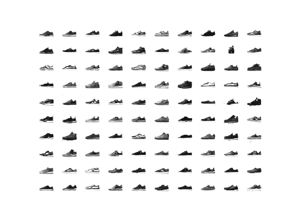
交流 GAN 生成的 100 张运动鞋照片示例
用其他类值进行实验可能会很有趣。
例如,下面是 100 个生成的涂层(n_class = 4)。大部分图像是外套,虽然里面有几条裤子,说明潜在空间是部分的,但不是完全的,有阶级条件的。

交流 GAN 生成涂层的 100 张照片示例
扩展ˌ扩张
本节列出了一些您可能希望探索的扩展教程的想法。
- 生成图像。为每个服装类别生成图像,并比较不同保存模型(例如纪元 10、20 等)的结果。).
- 备用配置。更新生成器、鉴别器或两种型号的配置,使其具有或多或少的容量并比较结果。
- CIFAR-10 数据集。更新示例以在 CIFAR-10 数据集上进行训练,并使用本文附录中描述的模型配置。
如果你探索这些扩展,我很想知道。
在下面的评论中发表你的发现。
进一步阅读
如果您想更深入地了解这个主题,本节将提供更多资源。
报纸
应用程序接口
- 硬数据集接口。
- Keras 顺序模型 API
- Keras 卷积层应用编程接口
- 如何“冻结”Keras 层?
- MatplotLib API
- NumPy 随机采样(numpy.random) API
- NumPy 数组操作例程
文章
摘要
在本教程中,您发现了如何开发一个辅助分类器生成对抗网络来生成服装照片。
具体来说,您了解到:
- 辅助分类器 GAN 是一种条件 GAN,它要求鉴别器预测给定图像的类别标签。
- 如何开发交流 GAN 的发生器、鉴别器和复合模型。
- 如何训练、评估和使用 AC-GAN 从时尚 MNIST 数据集生成服装照片。
你有什么问题吗?
在下面的评论中提问,我会尽力回答。
如何在 Keras 开发信息最大化 GAN(InfoGAN)
最后更新于 2021 年 1 月 18 日
生成对抗网络是一种用于训练深度卷积模型以生成合成图像的体系结构。
尽管非常有效,但默认的 GAN 无法控制生成的图像类型。信息最大化 GAN,简称 InfoGAN,是 GAN 架构的扩展,它引入了由架构自动学习的控制变量,并允许对生成的图像进行控制,例如在生成手写数字图像的情况下的样式、厚度和类型。
在本教程中,您将发现如何从零开始实现信息最大化生成对抗网络模型。
完成本教程后,您将知道:
- InfoGAN 的动机是希望解开和控制生成图像中的属性。
- InfoGAN 包括添加控制变量,以生成预测控制变量的辅助模型,该模型通过相互信息损失函数进行训练。
- 如何从零开始开发和训练一个 InfoGAN 模型,并使用控制变量来控制模型生成哪个数字。
用我的新书Python 生成对抗网络启动你的项目,包括分步教程和所有示例的 Python 源代码文件。
我们开始吧。
- 2019 年 10 月更新:修正了相互信息丢失解释中的错别字。
- 2021 年 1 月更新:更新了所以层冻结用批量定额工作。

如何在 Keras 开发一个信息最大化的生成对抗网络(InfoGAN)图片由伊罗尔·特拉蒙特提供,版权所有。
教程概述
本教程分为四个部分;它们是:
- 什么是信息最大化
- 如何实现信息增益损耗函数
- 如何为 MNIST 开发信息甘
- 如何使用训练有素的信息甘模型的控制代码
什么是信息最大化
生成对抗网络,简称 GAN,是一种用于训练生成模型的架构,例如用于生成合成图像的模型。
它包括用鉴别器模型同时训练用于生成图像的生成器模型,该鉴别器模型学习将图像分类为真实的(来自训练数据集)或虚假的(生成的)。这两个模型在零和游戏中竞争,因此训练过程的收敛包括在生成器生成令人信服的图像的技能和鉴别器检测图像的能力之间找到平衡。
生成器模型将潜在空间中的随机点作为输入,通常是 50 到 100 个随机高斯变量。生成器通过训练对潜在空间中的点应用唯一的含义,并将点映射到特定的输出合成图像。这意味着,尽管潜在空间是由生成器模型构造的,但是对生成的图像没有控制。
GAN 公式使用简单的因子化连续输入噪声矢量 z,同时对发生器使用该噪声的方式没有限制。因此,噪声可能会被生成器以高度纠缠的方式使用,导致 z 的各个维度与数据的语义特征不一致。
——InfoGAN:通过信息最大化生成对抗网进行可解释表征学习,2016。
可以探索潜在空间并比较生成的图像,以试图理解生成器模型已经学习的映射。或者,可以对生成过程进行调节,例如通过类别标签,以便可以按需创建特定类型的图像。这是条件生成对抗网络的基础。
另一种方法是提供控制变量作为发生器的输入,以及潜在空间中的点(噪声)。可以训练生成器使用控制变量来影响生成图像的特定属性。这是信息最大化生成对抗网络(简称 InfoGAN)采用的方法。
InfoGAN,生成对抗网络的信息论扩展,能够以完全无监督的方式学习不纠缠的表示。
——InfoGAN:通过信息最大化生成对抗网进行可解释表征学习,2016。
生成器在训练过程中学习的结构化映射有些随机。尽管生成器模型学习在潜在空间中空间分离生成的图像的属性,但是没有控制。性质是纠缠的。InfoGAN 的动机是希望解开生成图像的属性。
例如,在面的情况下,生成面的属性可以被解开和控制,例如面的形状、头发颜色、发型等等。
例如,对于人脸数据集,有用的解纠结表示可以为以下属性中的每一个分配单独的维度集:面部表情、眼睛颜色、发型、有无眼镜以及相应人的身份。
——InfoGAN:通过信息最大化生成对抗网进行可解释表征学习,2016。
控制变量与噪声一起作为输入提供给发生器,模型通过互信息损失函数进行训练。
……我们对生成对抗网络目标提出了一个简单的修改,鼓励它学习可解释和有意义的表示。我们通过最大化 GAN 噪声变量的固定小子集和观测值之间的互信息来做到这一点,这被证明是相对简单的。
——InfoGAN:通过信息最大化生成对抗网进行可解释表征学习,2016。
互信息是指在给定一个变量的情况下,对另一个变量所学习的信息量。在这种情况下,给定使用噪声和控制变量生成的图像,我们对关于控制变量的信息感兴趣。
在信息论中,X 和 Y 之间的互信息,I(X;Y),衡量从随机变量 Y 关于另一个随机变量 x 的知识中学到的“信息量
互信息(MI)计算为给定图像的控制变量©的条件熵(由生成器(G)从噪声(z)和控制变量©中创建)减去控制变量©的边缘熵;例如:
- MI =熵©–熵©;G(z,c))
实际上,计算真实的互信息通常是困难的,尽管本文采用了简化的方法,称为变分信息最大化,并且控制码的熵保持不变。有关相互信息的更多信息,请参见教程:
通过相互信息训练发电机是通过使用一个新的模型,称为 Q 或辅助模型来实现的。新模型与用于解释输入图像的鉴别器模型共享所有相同的权重,但是与预测图像是真还是假的鉴别器模型不同,辅助模型预测用于生成图像的控制代码。
这两个模型都用于更新生成器模型,首先是为了提高生成欺骗鉴别器模型的图像的可能性,其次是为了提高用于生成图像的控制代码和辅助模型对控制代码的预测之间的互信息。
结果是,生成器模型通过互信息损失被正则化,使得控制代码捕获生成的图像的显著属性,并且反过来可以用于控制图像生成过程。
……只要我们有兴趣学习从给定输入 X 到保留原始输入信息的更高级表示 Y 的参数化映射,就可以利用互信息。[……]表明最大化互信息的任务本质上等同于训练自动编码器以最小化重构误差。
——了解互信息及其在 InfoGAN 中的使用,2016。
如何实现信息增益损耗函数
一旦您熟悉了模型的输入和输出,InfoGAN 就相当容易实现了。
唯一的绊脚石可能是相互信息丢失函数,尤其是如果你没有像大多数开发人员那样强大的数学背景。
InfoGan 使用的控制变量主要有两种类型:分类变量和连续变量,连续变量可能具有不同的数据分布,这会影响相互损失的计算方式。基于变量类型,可以跨所有控制变量计算和求和相互损失,这是 OpenAI 为 TensorFlow 发布的官方 InfoGAN 实现中使用的方法。
在 Keras 中,可能更容易将控制变量简化为分类变量和高斯或均匀连续变量,并在辅助模型上为每种控制变量类型提供单独的输出。这样可以使用不同的损耗函数,大大简化了实现。
请参阅“进一步阅读”部分的文章和帖子,了解本部分建议的更多背景信息。
分类控制变量
分类变量可用于控制生成图像的类型或类别。
这被实现为一个热编码向量。也就是说,如果该类有 10 个值,那么控制代码将是一个类,例如 6,并且生成器模型的分类控制向量输入将是所有零值的 10 元素向量,对于类 6 具有 1 个值,例如[0,0,0,0,0,0,0,1,0,0]。
在训练模型时,我们不需要选择分类控制变量;取而代之的是,它们是随机生成的,例如,每个样本以统一的概率被选择。
……潜在码 c∞Cat 上的一致分类分布(K = 10,p = 0.1)
——InfoGAN:通过信息最大化生成对抗网进行可解释表征学习,2016。
在辅助模型中,分类变量的输出层也将是一个热编码向量,以匹配输入控制代码,并使用 softmax 激活函数。
对于分类潜在码 ci,我们使用 softmax 非线性的自然选择来表示 Q(ci |x)。
——InfoGAN:通过信息最大化生成对抗网进行可解释表征学习,2016。
回想一下,互信息被计算为来自控制变量的条件熵,以及从提供给输入变量的控制变量的熵中减去辅助模型的输出。我们可以直接实现这个,但是没有必要。
控制变量的熵是一个常数,结果是一个非常小的接近于零的数字;因此,我们可以将其从我们的计算中移除。条件熵可以直接计算为控制变量输入和辅助模型输出之间的交叉熵。因此,可以使用分类交叉熵损失函数,就像我们对任何多类分类问题一样。
超参数 lambda 用于缩放互信息损失函数,并设置为 1,因此可以忽略。
即使 InfoGAN 引入了一个额外的超参数λ,它也很容易调整,简单地设置为 1 就足以处理离散的潜在代码。
——InfoGAN:通过信息最大化生成对抗网进行可解释表征学习,2016。
连续控制变量
连续控制变量可用于控制图像的风格。
连续变量从均匀分布(例如-1 和 1 之间)中采样,并作为输入提供给生成器模型。
…能够捕捉本质上连续变化的连续代码:c2,C3∞Unif(1,1)
——InfoGAN:通过信息最大化生成对抗网进行可解释表征学习,2016。
辅助模型可以实现对具有高斯分布的连续控制变量的预测,其中输出层被配置为具有一个节点,即平均值,和一个高斯标准差的节点,例如每个连续控制变量需要两个输出。
对于连续潜在码 cj,取决于什么是真正的后验 P(cj |x),有更多的选择。在我们的实验中,我们发现简单地将 Q(cj |x)视为因子化高斯就足够了。
——InfoGAN:通过信息最大化生成对抗网进行可解释表征学习,2016。
输出平均值的节点可以使用线性激活函数,而输出标准差的节点必须产生正值,因此可以使用激活函数(如 sigmoid)来创建 0 到 1 之间的值。
对于连续潜在码,我们通过对角高斯分布参数化近似后验,识别网络输出其均值和标准差,其中标准差通过网络输出的指数变换参数化以确保正定性。
——InfoGAN:通过信息最大化生成对抗网进行可解释表征学习,2016。
损失函数必须作为高斯控制码的互信息来计算,这意味着在计算损失之前,必须根据平均值和标准偏差来重构它们。计算高斯分布变量的熵和条件熵可以直接实现,尽管不是必须的。相反,可以使用均方误差损失。
或者,输出分布可以简化为每个控制变量的均匀分布,可以使用具有线性激活的辅助模型中每个变量的单个输出节点,并且模型可以使用均方误差损失函数。
如何为 MNIST 开发信息甘
在这一节中,我们将仔细研究生成器(g)、鉴别器(d)和辅助模型(q)以及如何在 Keras 中实现它们。
我们将为 MNIST 数据集开发一个 InfoGAN 实现,正如 InfoGAN 论文中所做的那样。
本文探讨了两个版本;第一种只使用分类控制代码,允许模型将一个分类变量映射到大约一个数字(尽管没有分类变量对数字的排序)。
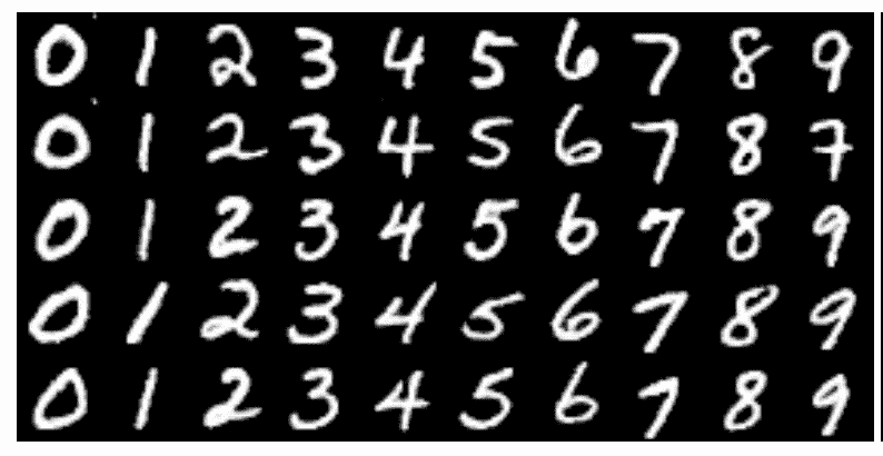
通过类别控制代码的值改变生成数字的示例。
摘自 InfoGan 论文。
本文还探讨了 InfoGAN 架构的一个版本,其中包含一个热编码分类变量(c1)和两个连续控制变量(c2 和 c3)。
发现第一个连续变量控制手指的旋转,第二个变量控制手指的粗细。
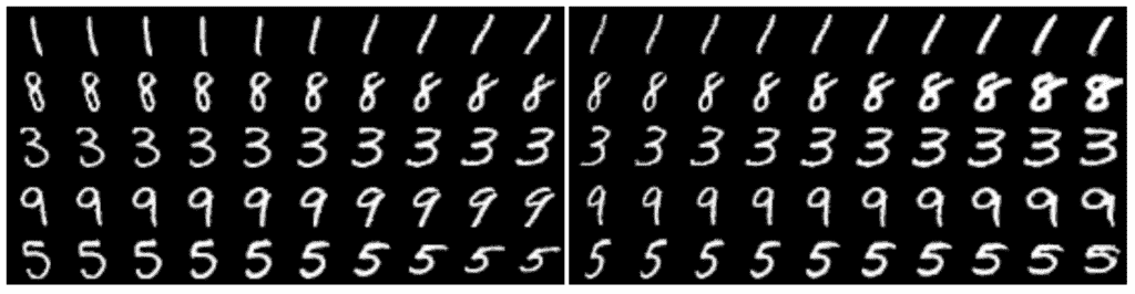
使用连续控制代码改变生成的数字倾斜度和厚度的示例。
摘自 InfoGan 论文。
我们将关注使用具有 10 个值的分类控制变量的简单情况,并鼓励模型学习让这个变量控制生成的数字。您可能希望通过更改分类控制变量的基数或添加连续控制变量来扩展这个示例。
用于在 MNIST 数据集上进行训练的全球导航卫星系统模型的配置作为该文件的附录提供,转载如下。我们将使用列出的配置作为开发我们自己的生成器(g)、鉴别器(d)和辅助(q)模型的起点。

MNIST 训练信息网的发生器、鉴别器和辅助模型配置总结。
摘自 InfoGan 论文。
让我们从将生成器模型开发为深度卷积神经网络(例如 DCGAN)开始。
该模型可以将噪声向量(z)和控制向量©作为单独的输入,并在将它们用作生成图像的基础之前将它们连接起来。或者,可以预先将向量连接起来,并提供给模型中的单个输入层。这两种方法是等效的,在这种情况下,我们将使用后者来保持模型简单。
下面的 define_generator() 函数定义了生成器模型,并将输入向量的大小作为参数。
一个完全连通的层获取输入向量,并产生足够数量的激活,以创建 512 个 7×7 的特征图,从这些特征图中激活被重塑。然后,这些通过具有 1×1 步距的正常卷积层,然后两个后续的上放大以 2×2 步距将卷积层首先转置到 14×14 特征映射,然后通过 tanh 激活函数转置到像素值在[-1,-1]范围内的期望 1 通道 28×28 特征映射输出。
好的生成器配置试探法如下,包括随机高斯权重初始化、隐藏层中的 ReLU 激活,以及使用批量归一化。
# define the standalone generator model
def define_generator(gen_input_size):
	# weight initialization
	init = RandomNormal(stddev=0.02)
	# image generator input
	in_lat = Input(shape=(gen_input_size,))
	# foundation for 7x7 image
	n_nodes = 512 * 7 * 7
	gen = Dense(n_nodes, kernel_initializer=init)(in_lat)
	gen = Activation('relu')(gen)
	gen = BatchNormalization()(gen)
	gen = Reshape((7, 7, 512))(gen)
	# normal
	gen = Conv2D(128, (4,4), padding='same', kernel_initializer=init)(gen)
	gen = Activation('relu')(gen)
	gen = BatchNormalization()(gen)
	# upsample to 14x14
	gen = Conv2DTranspose(64, (4,4), strides=(2,2), padding='same', kernel_initializer=init)(gen)
	gen = Activation('relu')(gen)
	gen = BatchNormalization()(gen)
	# upsample to 28x28
	gen = Conv2DTranspose(1, (4,4), strides=(2,2), padding='same', kernel_initializer=init)(gen)
	# tanh output
	out_layer = Activation('tanh')(gen)
	# define model
	model = Model(in_lat, out_layer)
	return model
接下来,我们可以定义鉴别器和辅助模型。
鉴别器模型以独立的方式在真实和虚假图像上进行训练,就像普通的 GAN 一样。发电机和辅助模型都不直接匹配;相反,它们适合作为复合模型的一部分。
鉴别器和辅助模型共享相同的输入和特征提取层,但输出层不同。因此,同时定义它们是有意义的。
同样,这种体系结构有许多实现方式,但是首先将鉴别器和辅助模型定义为单独的模型允许我们稍后通过功能 API 直接将它们组合成一个更大的 GAN 模型。
下面的 define_discriminator() 函数定义了鉴别器和辅助模型,并将分类变量的基数(例如数值的个数,如 10)作为输入。输入图像的形状也被参数化为函数参数,并设置为 MNIST 图像大小的默认值。
特征提取层涉及两个下采样层,作为最佳实践,使用这两个下采样层代替池化层。同样遵循 DCGAN 模型的最佳实践,我们使用 LeakyReLU 激活和批处理规范化。
鉴别器模型(d)具有单个输出节点,并通过 sigmoid 激活函数预测输入图像真实的概率。该模型将独立使用,通过具有最佳实践学习率和动量的随机梯度下降的亚当版本优化二元交叉熵函数。
辅助模型(q)对于分类变量中的每个值都有一个节点输出,并使用 softmax 激活函数。像 InfoGAN 论文中使用的那样,在特征提取层和输出层之间添加了一个完全连接的层。模型不会被编译,因为它不是以独立的方式形成或使用的。
# define the standalone discriminator model
def define_discriminator(n_cat, in_shape=(28,28,1)):
	# weight initialization
	init = RandomNormal(stddev=0.02)
	# image input
	in_image = Input(shape=in_shape)
	# downsample to 14x14
	d = Conv2D(64, (4,4), strides=(2,2), padding='same', kernel_initializer=init)(in_image)
	d = LeakyReLU(alpha=0.1)(d)
	# downsample to 7x7
	d = Conv2D(128, (4,4), strides=(2,2), padding='same', kernel_initializer=init)(d)
	d = LeakyReLU(alpha=0.1)(d)
	d = BatchNormalization()(d)
	# normal
	d = Conv2D(256, (4,4), padding='same', kernel_initializer=init)(d)
	d = LeakyReLU(alpha=0.1)(d)
	d = BatchNormalization()(d)
	# flatten feature maps
	d = Flatten()(d)
	# real/fake output
	out_classifier = Dense(1, activation='sigmoid')(d)
	# define d model
	d_model = Model(in_image, out_classifier)
	# compile d model
	d_model.compile(loss='binary_crossentropy', optimizer=Adam(lr=0.0002, beta_1=0.5))
	# create q model layers
	q = Dense(128)(d)
	q = BatchNormalization()(q)
	q = LeakyReLU(alpha=0.1)(q)
	# q model output
	out_codes = Dense(n_cat, activation='softmax')(q)
	# define q model
	q_model = Model(in_image, out_codes)
	return d_model, q_model
接下来,我们可以定义复合 GAN 模型。
该模型使用所有子模型,并且是训练生成器模型的权重的基础。
下面的 define_gan() 函数实现了这一点,定义并返回模型,将三个子模型作为输入。
如上所述,鉴别器是以独立方式训练的,因此鉴别器的所有权重都被设置为不可训练(仅在本文中)。生成器模型的输出连接到鉴别器模型的输入和辅助模型的输入。
这将创建一个新的复合模型,该模型将[噪声+控制]向量作为输入,然后通过生成器生成图像。图像然后通过鉴别器模型产生分类,并通过辅助模型产生控制变量的预测。
该模型有两个输出层,需要用不同的损失函数进行训练。二进制交叉熵损失用于鉴别器输出,正如我们在编译独立使用的鉴别器时所做的那样,互信息损失用于辅助模型,在这种情况下,辅助模型可以直接实现为分类交叉熵,并获得期望的结果。
# define the combined discriminator, generator and q network model
def define_gan(g_model, d_model, q_model):
	# make weights in the discriminator (some shared with the q model) as not trainable
	for layer in d_model.layers:
		if not isinstance(layer, BatchNormalization):
			layer.trainable = False
	# connect g outputs to d inputs
	d_output = d_model(g_model.output)
	# connect g outputs to q inputs
	q_output = q_model(g_model.output)
	# define composite model
	model = Model(g_model.input, [d_output, q_output])
	# compile model
	opt = Adam(lr=0.0002, beta_1=0.5)
	model.compile(loss=['binary_crossentropy', 'categorical_crossentropy'], optimizer=opt)
	return model
为了使 GAN 模型架构更加清晰,我们可以创建模型和复合模型的图。
下面列出了完整的示例。
# create and plot the infogan model for mnist
from keras.optimizers import Adam
from keras.models import Model
from keras.layers import Input
from keras.layers import Dense
from keras.layers import Reshape
from keras.layers import Flatten
from keras.layers import Conv2D
from keras.layers import Conv2DTranspose
from keras.layers import LeakyReLU
from keras.layers import BatchNormalization
from keras.layers import Activation
from keras.initializers import RandomNormal
from keras.utils.vis_utils import plot_model

# define the standalone discriminator model
def define_discriminator(n_cat, in_shape=(28,28,1)):
	# weight initialization
	init = RandomNormal(stddev=0.02)
	# image input
	in_image = Input(shape=in_shape)
	# downsample to 14x14
	d = Conv2D(64, (4,4), strides=(2,2), padding='same', kernel_initializer=init)(in_image)
	d = LeakyReLU(alpha=0.1)(d)
	# downsample to 7x7
	d = Conv2D(128, (4,4), strides=(2,2), padding='same', kernel_initializer=init)(d)
	d = LeakyReLU(alpha=0.1)(d)
	d = BatchNormalization()(d)
	# normal
	d = Conv2D(256, (4,4), padding='same', kernel_initializer=init)(d)
	d = LeakyReLU(alpha=0.1)(d)
	d = BatchNormalization()(d)
	# flatten feature maps
	d = Flatten()(d)
	# real/fake output
	out_classifier = Dense(1, activation='sigmoid')(d)
	# define d model
	d_model = Model(in_image, out_classifier)
	# compile d model
	d_model.compile(loss='binary_crossentropy', optimizer=Adam(lr=0.0002, beta_1=0.5))
	# create q model layers
	q = Dense(128)(d)
	q = BatchNormalization()(q)
	q = LeakyReLU(alpha=0.1)(q)
	# q model output
	out_codes = Dense(n_cat, activation='softmax')(q)
	# define q model
	q_model = Model(in_image, out_codes)
	return d_model, q_model

# define the standalone generator model
def define_generator(gen_input_size):
	# weight initialization
	init = RandomNormal(stddev=0.02)
	# image generator input
	in_lat = Input(shape=(gen_input_size,))
	# foundation for 7x7 image
	n_nodes = 512 * 7 * 7
	gen = Dense(n_nodes, kernel_initializer=init)(in_lat)
	gen = Activation('relu')(gen)
	gen = BatchNormalization()(gen)
	gen = Reshape((7, 7, 512))(gen)
	# normal
	gen = Conv2D(128, (4,4), padding='same', kernel_initializer=init)(gen)
	gen = Activation('relu')(gen)
	gen = BatchNormalization()(gen)
	# upsample to 14x14
	gen = Conv2DTranspose(64, (4,4), strides=(2,2), padding='same', kernel_initializer=init)(gen)
	gen = Activation('relu')(gen)
	gen = BatchNormalization()(gen)
	# upsample to 28x28
	gen = Conv2DTranspose(1, (4,4), strides=(2,2), padding='same', kernel_initializer=init)(gen)
	# tanh output
	out_layer = Activation('tanh')(gen)
	# define model
	model = Model(in_lat, out_layer)
	return model

# define the combined discriminator, generator and q network model
def define_gan(g_model, d_model, q_model):
	# make weights in the discriminator (some shared with the q model) as not trainable
	for layer in d_model.layers:
		if not isinstance(layer, BatchNormalization):
			layer.trainable = False
	# connect g outputs to d inputs
	d_output = d_model(g_model.output)
	# connect g outputs to q inputs
	q_output = q_model(g_model.output)
	# define composite model
	model = Model(g_model.input, [d_output, q_output])
	# compile model
	opt = Adam(lr=0.0002, beta_1=0.5)
	model.compile(loss=['binary_crossentropy', 'categorical_crossentropy'], optimizer=opt)
	return model

# number of values for the categorical control code
n_cat = 10
# size of the latent space
latent_dim = 62
# create the discriminator
d_model, q_model = define_discriminator(n_cat)
# create the generator
gen_input_size = latent_dim + n_cat
g_model = define_generator(gen_input_size)
# create the gan
gan_model = define_gan(g_model, d_model, q_model)
# plot the model
plot_model(gan_model, to_file='gan_plot.png', show_shapes=True, show_layer_names=True)
运行该示例会创建所有三个模型,然后创建复合 GAN 模型并保存模型体系结构图。
注:创建此图假设安装了 pydot 和 graphviz 库。如果这是一个问题,您可以注释掉导入语句和对 plot_model() 函数的调用。
该图显示了生成器模型的所有细节以及鉴别器和辅助模型的压缩描述。重要的是,注意鉴别器输出的形状,作为预测图像是真还是假的单个节点,10 个节点用于辅助模型来预测分类控制代码。
回想一下,该复合模型将仅用于更新生成器和辅助模型的模型权重,并且鉴别器模型中的所有权重将保持不可跟踪,即仅在独立鉴别器模型更新时更新。
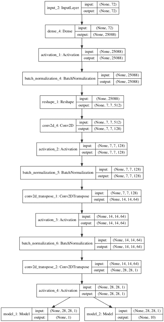
用于训练发电机和辅助模型的复合信息甘模型图
接下来,我们将开发发电机的输入。
每个输入都是由噪声和控制代码组成的矢量。具体来说,高斯随机数的向量和一个热编码随机选择的分类值。
下面的generate _ 潜伏 _points() 函数实现了这一点,将潜伏空间的大小、分类值的数量和要生成的样本数量作为参数作为输入。该函数返回输入串联矢量作为发电机模型的输入,以及独立控制代码。当通过复合 GAN 模型更新发电机和辅助模型时,将需要独立的控制代码,特别是用于计算辅助模型的相互信息损失。
# generate points in latent space as input for the generator
def generate_latent_points(latent_dim, n_cat, n_samples):
	# generate points in the latent space
	z_latent = randn(latent_dim * n_samples)
	# reshape into a batch of inputs for the network
	z_latent = z_latent.reshape(n_samples, latent_dim)
	# generate categorical codes
	cat_codes = randint(0, n_cat, n_samples)
	# one hot encode
	cat_codes = to_categorical(cat_codes, num_classes=n_cat)
	# concatenate latent points and control codes
	z_input = hstack((z_latent, cat_codes))
	return [z_input, cat_codes]
接下来,我们可以生成真实和虚假的例子。
可以加载 MNIST 数据集,通过为灰度图像添加额外的维度并将所有像素值缩放到范围[-1,1]以匹配生成器模型的输出,将其转换为 3D 输入。这在下面的 load_real_samples() 函数中实现。
我们可以通过选择数据集的随机子集来检索训练鉴别器时所需的真实样本批次。这在下面的 generate_real_samples() 函数中实现,该函数返回图像和类别标签 1,以向鉴别器指示它们是真实图像。
鉴别器还需要通过生成器生成成批的假样本,使用来自generate _ 潜伏 _points() 函数的向量作为输入。下面的 generate_fake_samples() 函数实现了这一点,返回生成的图像以及类标签 0,以向鉴别器指示它们是假图像。
# load images
def load_real_samples():
	# load dataset
	(trainX, _), (_, _) = load_data()
	# expand to 3d, e.g. add channels
	X = expand_dims(trainX, axis=-1)
	# convert from ints to floats
	X = X.astype('float32')
	# scale from [0,255] to [-1,1]
	X = (X - 127.5) / 127.5
	print(X.shape)
	return X

# select real samples
def generate_real_samples(dataset, n_samples):
	# choose random instances
	ix = randint(0, dataset.shape[0], n_samples)
	# select images and labels
	X = dataset[ix]
	# generate class labels
	y = ones((n_samples, 1))
	return X, y

# use the generator to generate n fake examples, with class labels
def generate_fake_samples(generator, latent_dim, n_cat, n_samples):
	# generate points in latent space and control codes
	z_input, _ = generate_latent_points(latent_dim, n_cat, n_samples)
	# predict outputs
	images = generator.predict(z_input)
	# create class labels
	y = zeros((n_samples, 1))
	return images, y
接下来,我们需要跟踪生成图像的质量。
我们将定期使用生成器生成图像样本,并将生成器和合成模型保存到文件中。然后,我们可以在训练结束时查看生成的图像,以便选择最终的生成器模型,并加载该模型以开始使用它来生成图像。
下面的*summary _ performance()*函数实现了这一点,首先生成 100 个图像,将它们的像素值缩放回范围[0,1],并将其保存为 10×10 平方的图像图。
生成器和复合 GAN 模型也保存到文件中,并根据训练迭代号使用唯一的文件名。
# generate samples and save as a plot and save the model
def summarize_performance(step, g_model, gan_model, latent_dim, n_cat, n_samples=100):
	# prepare fake examples
	X, _ = generate_fake_samples(g_model, latent_dim, n_cat, n_samples)
	# scale from [-1,1] to [0,1]
	X = (X + 1) / 2.0
	# plot images
	for i in range(100):
		# define subplot
		pyplot.subplot(10, 10, 1 + i)
		# turn off axis
		pyplot.axis('off')
		# plot raw pixel data
		pyplot.imshow(X[i, :, :, 0], cmap='gray_r')
	# save plot to file
	filename1 = 'generated_plot_%04d.png' % (step+1)
	pyplot.savefig(filename1)
	pyplot.close()
	# save the generator model
	filename2 = 'model_%04d.h5' % (step+1)
	g_model.save(filename2)
	# save the gan model
	filename3 = 'gan_model_%04d.h5' % (step+1)
	gan_model.save(filename3)
	print('>Saved: %s, %s, and %s' % (filename1, filename2, filename3))
最后,我们可以训练信息甘。
这在下面的 train() 函数中实现,该函数将定义的模型和配置作为参数并运行训练过程。
模型被训练了 100 个时期,每个批次使用 64 个样本。MNIST 训练数据集中有 60,000 幅图像,因此一个时期涉及 60,000/64,或 937 个批次或训练迭代。将其乘以纪元的数量,即 100,意味着总共将有 93,700 次训练迭代。
每次训练迭代都包括首先用半批真实样本和半批伪样本更新鉴别器,以在每次迭代中形成一批有价值的权重更新,即 64。接下来,基于一批有价值的噪声和控制代码输入来更新复合 GAN 模型。在每次训练迭代中报告真假图像鉴别器的损失以及生成器和辅助模型的损失。
# train the generator and discriminator
def train(g_model, d_model, gan_model, dataset, latent_dim, n_cat, n_epochs=100, n_batch=64):
	# calculate the number of batches per training epoch
	bat_per_epo = int(dataset.shape[0] / n_batch)
	# calculate the number of training iterations
	n_steps = bat_per_epo * n_epochs
	# calculate the size of half a batch of samples
	half_batch = int(n_batch / 2)
	# manually enumerate epochs
	for i in range(n_steps):
		# get randomly selected 'real' samples
		X_real, y_real = generate_real_samples(dataset, half_batch)
		# update discriminator and q model weights
		d_loss1 = d_model.train_on_batch(X_real, y_real)
		# generate 'fake' examples
		X_fake, y_fake = generate_fake_samples(g_model, latent_dim, n_cat, half_batch)
		# update discriminator model weights
		d_loss2 = d_model.train_on_batch(X_fake, y_fake)
		# prepare points in latent space as input for the generator
		z_input, cat_codes = generate_latent_points(latent_dim, n_cat, n_batch)
		# create inverted labels for the fake samples
		y_gan = ones((n_batch, 1))
		# update the g via the d and q error
		_,g_1,g_2 = gan_model.train_on_batch(z_input, [y_gan, cat_codes])
		# summarize loss on this batch
		print('>%d, d[%.3f,%.3f], g[%.3f] q[%.3f]' % (i+1, d_loss1, d_loss2, g_1, g_2))
		# evaluate the model performance every 'epoch'
		if (i+1) % (bat_per_epo * 10) == 0:
			summarize_performance(i, g_model, gan_model, latent_dim, n_cat)
然后,我们可以配置和创建模型,然后运行培训过程。
我们将使用单个分类变量的 10 个值来匹配 MNIST 数据集中的 10 个已知类。我们将使用 64 维的潜在空间来匹配 InfoGAN 论文,这意味着,在这种情况下,生成器模型的每个输入向量将是 64(随机高斯变量)+ 10(一个热编码控制变量)或 72 个元素的长度。
# number of values for the categorical control code
n_cat = 10
# size of the latent space
latent_dim = 62
# create the discriminator
d_model, q_model = define_discriminator(n_cat)
# create the generator
gen_input_size = latent_dim + n_cat
g_model = define_generator(gen_input_size)
# create the gan
gan_model = define_gan(g_model, d_model, q_model)
# load image data
dataset = load_real_samples()
# train model
train(g_model, d_model, gan_model, dataset, latent_dim, n_cat)
将这些联系在一起,下面列出了在 MNIST 数据集上使用单个分类控制变量训练 InfoGAN 模型的完整示例。
# example of training an infogan on mnist
from numpy import zeros
from numpy import ones
from numpy import expand_dims
from numpy import hstack
from numpy.random import randn
from numpy.random import randint
from keras.datasets.mnist import load_data
from keras.optimizers import Adam
from keras.initializers import RandomNormal
from keras.utils import to_categorical
from keras.models import Model
from keras.layers import Input
from keras.layers import Dense
from keras.layers import Reshape
from keras.layers import Flatten
from keras.layers import Conv2D
from keras.layers import Conv2DTranspose
from keras.layers import LeakyReLU
from keras.layers import BatchNormalization
from keras.layers import Activation
from matplotlib import pyplot

# define the standalone discriminator model
def define_discriminator(n_cat, in_shape=(28,28,1)):
	# weight initialization
	init = RandomNormal(stddev=0.02)
	# image input
	in_image = Input(shape=in_shape)
	# downsample to 14x14
	d = Conv2D(64, (4,4), strides=(2,2), padding='same', kernel_initializer=init)(in_image)
	d = LeakyReLU(alpha=0.1)(d)
	# downsample to 7x7
	d = Conv2D(128, (4,4), strides=(2,2), padding='same', kernel_initializer=init)(d)
	d = LeakyReLU(alpha=0.1)(d)
	d = BatchNormalization()(d)
	# normal
	d = Conv2D(256, (4,4), padding='same', kernel_initializer=init)(d)
	d = LeakyReLU(alpha=0.1)(d)
	d = BatchNormalization()(d)
	# flatten feature maps
	d = Flatten()(d)
	# real/fake output
	out_classifier = Dense(1, activation='sigmoid')(d)
	# define d model
	d_model = Model(in_image, out_classifier)
	# compile d model
	d_model.compile(loss='binary_crossentropy', optimizer=Adam(lr=0.0002, beta_1=0.5))
	# create q model layers
	q = Dense(128)(d)
	q = BatchNormalization()(q)
	q = LeakyReLU(alpha=0.1)(q)
	# q model output
	out_codes = Dense(n_cat, activation='softmax')(q)
	# define q model
	q_model = Model(in_image, out_codes)
	return d_model, q_model

# define the standalone generator model
def define_generator(gen_input_size):
	# weight initialization
	init = RandomNormal(stddev=0.02)
	# image generator input
	in_lat = Input(shape=(gen_input_size,))
	# foundation for 7x7 image
	n_nodes = 512 * 7 * 7
	gen = Dense(n_nodes, kernel_initializer=init)(in_lat)
	gen = Activation('relu')(gen)
	gen = BatchNormalization()(gen)
	gen = Reshape((7, 7, 512))(gen)
	# normal
	gen = Conv2D(128, (4,4), padding='same', kernel_initializer=init)(gen)
	gen = Activation('relu')(gen)
	gen = BatchNormalization()(gen)
	# upsample to 14x14
	gen = Conv2DTranspose(64, (4,4), strides=(2,2), padding='same', kernel_initializer=init)(gen)
	gen = Activation('relu')(gen)
	gen = BatchNormalization()(gen)
	# upsample to 28x28
	gen = Conv2DTranspose(1, (4,4), strides=(2,2), padding='same', kernel_initializer=init)(gen)
	# tanh output
	out_layer = Activation('tanh')(gen)
	# define model
	model = Model(in_lat, out_layer)
	return model

# define the combined discriminator, generator and q network model
def define_gan(g_model, d_model, q_model):
	# make weights in the discriminator (some shared with the q model) as not trainable
	for layer in d_model.layers:
		if not isinstance(layer, BatchNormalization):
			layer.trainable = False
	# connect g outputs to d inputs
	d_output = d_model(g_model.output)
	# connect g outputs to q inputs
	q_output = q_model(g_model.output)
	# define composite model
	model = Model(g_model.input, [d_output, q_output])
	# compile model
	opt = Adam(lr=0.0002, beta_1=0.5)
	model.compile(loss=['binary_crossentropy', 'categorical_crossentropy'], optimizer=opt)
	return model

# load images
def load_real_samples():
	# load dataset
	(trainX, _), (_, _) = load_data()
	# expand to 3d, e.g. add channels
	X = expand_dims(trainX, axis=-1)
	# convert from ints to floats
	X = X.astype('float32')
	# scale from [0,255] to [-1,1]
	X = (X - 127.5) / 127.5
	print(X.shape)
	return X

# select real samples
def generate_real_samples(dataset, n_samples):
	# choose random instances
	ix = randint(0, dataset.shape[0], n_samples)
	# select images and labels
	X = dataset[ix]
	# generate class labels
	y = ones((n_samples, 1))
	return X, y

# generate points in latent space as input for the generator
def generate_latent_points(latent_dim, n_cat, n_samples):
	# generate points in the latent space
	z_latent = randn(latent_dim * n_samples)
	# reshape into a batch of inputs for the network
	z_latent = z_latent.reshape(n_samples, latent_dim)
	# generate categorical codes
	cat_codes = randint(0, n_cat, n_samples)
	# one hot encode
	cat_codes = to_categorical(cat_codes, num_classes=n_cat)
	# concatenate latent points and control codes
	z_input = hstack((z_latent, cat_codes))
	return [z_input, cat_codes]

# use the generator to generate n fake examples, with class labels
def generate_fake_samples(generator, latent_dim, n_cat, n_samples):
	# generate points in latent space and control codes
	z_input, _ = generate_latent_points(latent_dim, n_cat, n_samples)
	# predict outputs
	images = generator.predict(z_input)
	# create class labels
	y = zeros((n_samples, 1))
	return images, y

# generate samples and save as a plot and save the model
def summarize_performance(step, g_model, gan_model, latent_dim, n_cat, n_samples=100):
	# prepare fake examples
	X, _ = generate_fake_samples(g_model, latent_dim, n_cat, n_samples)
	# scale from [-1,1] to [0,1]
	X = (X + 1) / 2.0
	# plot images
	for i in range(100):
		# define subplot
		pyplot.subplot(10, 10, 1 + i)
		# turn off axis
		pyplot.axis('off')
		# plot raw pixel data
		pyplot.imshow(X[i, :, :, 0], cmap='gray_r')
	# save plot to file
	filename1 = 'generated_plot_%04d.png' % (step+1)
	pyplot.savefig(filename1)
	pyplot.close()
	# save the generator model
	filename2 = 'model_%04d.h5' % (step+1)
	g_model.save(filename2)
	# save the gan model
	filename3 = 'gan_model_%04d.h5' % (step+1)
	gan_model.save(filename3)
	print('>Saved: %s, %s, and %s' % (filename1, filename2, filename3))

# train the generator and discriminator
def train(g_model, d_model, gan_model, dataset, latent_dim, n_cat, n_epochs=100, n_batch=64):
	# calculate the number of batches per training epoch
	bat_per_epo = int(dataset.shape[0] / n_batch)
	# calculate the number of training iterations
	n_steps = bat_per_epo * n_epochs
	# calculate the size of half a batch of samples
	half_batch = int(n_batch / 2)
	# manually enumerate epochs
	for i in range(n_steps):
		# get randomly selected 'real' samples
		X_real, y_real = generate_real_samples(dataset, half_batch)
		# update discriminator and q model weights
		d_loss1 = d_model.train_on_batch(X_real, y_real)
		# generate 'fake' examples
		X_fake, y_fake = generate_fake_samples(g_model, latent_dim, n_cat, half_batch)
		# update discriminator model weights
		d_loss2 = d_model.train_on_batch(X_fake, y_fake)
		# prepare points in latent space as input for the generator
		z_input, cat_codes = generate_latent_points(latent_dim, n_cat, n_batch)
		# create inverted labels for the fake samples
		y_gan = ones((n_batch, 1))
		# update the g via the d and q error
		_,g_1,g_2 = gan_model.train_on_batch(z_input, [y_gan, cat_codes])
		# summarize loss on this batch
		print('>%d, d[%.3f,%.3f], g[%.3f] q[%.3f]' % (i+1, d_loss1, d_loss2, g_1, g_2))
		# evaluate the model performance every 'epoch'
		if (i+1) % (bat_per_epo * 10) == 0:
			summarize_performance(i, g_model, gan_model, latent_dim, n_cat)

# number of values for the categorical control code
n_cat = 10
# size of the latent space
latent_dim = 62
# create the discriminator
d_model, q_model = define_discriminator(n_cat)
# create the generator
gen_input_size = latent_dim + n_cat
g_model = define_generator(gen_input_size)
# create the gan
gan_model = define_gan(g_model, d_model, q_model)
# load image data
dataset = load_real_samples()
# train model
train(g_model, d_model, gan_model, dataset, latent_dim, n_cat)
运行示例可能需要一些时间,建议使用 GPU 硬件,但不是必需的。
注:考虑到算法或评估程序的随机性,或数值准确率的差异,您的结果可能会有所不同。考虑运行该示例几次,并比较平均结果。
在每次训练迭代中报告模型间的损失。如果鉴别器的损失保持在 0.0 或长时间达到 0.0,这可能是训练失败的信号,您可能需要重新开始训练过程。鉴别器损耗可能从 0.0 开始,但很可能会上升,就像在这种特定情况下一样。
辅助模型的损失可能会为零,因为它完美地预测了分类变量。生成器和鉴别器模型的损失最终可能会在 1.0 左右徘徊,以证明两个模型的训练过程稳定或平衡。
>1, d[0.924,0.758], g[0.448] q[2.909]
>2, d[0.000,2.699], g[0.547] q[2.704]
>3, d[0.000,1.557], g[1.175] q[2.820]
>4, d[0.000,0.941], g[1.466] q[2.813]
>5, d[0.000,1.013], g[1.908] q[2.715]
...
>93696, d[0.814,1.212], g[1.283] q[0.000]
>93697, d[1.063,0.920], g[1.132] q[0.000]
>93698, d[0.999,1.188], g[1.128] q[0.000]
>93699, d[0.935,0.985], g[1.229] q[0.000]
>93700, d[0.968,1.016], g[1.200] q[0.001]
>Saved: generated_plot_93700.png, model_93700.h5, and gan_model_93700.h5
绘图和模型每 10 个时代或每 9370 次训练迭代保存一次。
审查图应显示早期的低质量图像和后期的改进和稳定质量图像。
例如,前 10 个纪元后保存的图像图如下,显示了低质量生成的图像。

信息甘在 10 个训练阶段后生成的 100 幅随机图像图
更多的时期并不意味着更好的质量,这意味着质量最好的图像可能不是那些在训练结束时保存的最终模型的图像。
查看图并选择具有最佳图像质量的最终模型。在这种情况下,我们将使用 100 个时代或 93,700 次训练迭代后保存的模型。

InfoGAN 在 100 个训练时期后生成的 100 幅随机图像的绘图
如何使用训练有素的信息甘模型的控制代码
现在我们已经训练了 InfoGAN 模型,我们可以探索如何使用它。
首先,我们可以加载模型,并使用它来生成随机图像,就像我们在训练期间所做的那样。
下面列出了完整的示例。
更改模型文件名,使其与训练运行期间生成最佳图像的模型文件名相匹配。
# example of loading the generator model and generating images
from math import sqrt
from numpy import hstack
from numpy.random import randn
from numpy.random import randint
from keras.models import load_model
from keras.utils import to_categorical
from matplotlib import pyplot

# generate points in latent space as input for the generator
def generate_latent_points(latent_dim, n_cat, n_samples):
	# generate points in the latent space
	z_latent = randn(latent_dim * n_samples)
	# reshape into a batch of inputs for the network
	z_latent = z_latent.reshape(n_samples, latent_dim)
	# generate categorical codes
	cat_codes = randint(0, n_cat, n_samples)
	# one hot encode
	cat_codes = to_categorical(cat_codes, num_classes=n_cat)
	# concatenate latent points and control codes
	z_input = hstack((z_latent, cat_codes))
	return [z_input, cat_codes]

# create a plot of generated images
def create_plot(examples, n_examples):
	# plot images
	for i in range(n_examples):
		# define subplot
		pyplot.subplot(sqrt(n_examples), sqrt(n_examples), 1 + i)
		# turn off axis
		pyplot.axis('off')
		# plot raw pixel data
		pyplot.imshow(examples[i, :, :, 0], cmap='gray_r')
	pyplot.show()

# load model
model = load_model('model_93700.h5')
# number of values for the categorical control code
n_cat = 10
# size of the latent space
latent_dim = 62
# number of examples to generate
n_samples = 100
# generate points in latent space and control codes
z_input, _ = generate_latent_points(latent_dim, n_cat, n_samples)
# predict outputs
X = model.predict(z_input)
# scale from [-1,1] to [0,1]
X = (X + 1) / 2.0
# plot the result
create_plot(X, n_samples)
运行该示例将加载保存的生成器模型,并使用它生成 100 个随机图像,并将图像绘制在 10×10 的网格上。

通过加载保存的信息甘生成器模型创建的 100 幅随机图像图
接下来,我们可以更新这个例子来测试我们的控制变量给了我们多少控制。
我们可以更新generate _ 潜伏 _points() 函数,获取[0,9]中分类值的参数值,对其进行编码,并将其与噪声向量一起用作输入。
# generate points in latent space as input for the generator
def generate_latent_points(latent_dim, n_cat, n_samples, digit):
	# generate points in the latent space
	z_latent = randn(latent_dim * n_samples)
	# reshape into a batch of inputs for the network
	z_latent = z_latent.reshape(n_samples, latent_dim)
	# define categorical codes
	cat_codes = asarray([digit for _ in range(n_samples)])
	# one hot encode
	cat_codes = to_categorical(cat_codes, num_classes=n_cat)
	# concatenate latent points and control codes
	z_input = hstack((z_latent, cat_codes))
	return [z_input, cat_codes]
我们可以通过生成分类值为 1 的 25 幅图像的网格来测试这一点。
下面列出了完整的示例。
# example of testing different values of the categorical control variable
from math import sqrt
from numpy import asarray
from numpy import hstack
from numpy.random import randn
from numpy.random import randint
from keras.models import load_model
from keras.utils import to_categorical
from matplotlib import pyplot

# generate points in latent space as input for the generator
def generate_latent_points(latent_dim, n_cat, n_samples, digit):
	# generate points in the latent space
	z_latent = randn(latent_dim * n_samples)
	# reshape into a batch of inputs for the network
	z_latent = z_latent.reshape(n_samples, latent_dim)
	# define categorical codes
	cat_codes = asarray([digit for _ in range(n_samples)])
	# one hot encode
	cat_codes = to_categorical(cat_codes, num_classes=n_cat)
	# concatenate latent points and control codes
	z_input = hstack((z_latent, cat_codes))
	return [z_input, cat_codes]

# create and save a plot of generated images
def save_plot(examples, n_examples):
	# plot images
	for i in range(n_examples):
		# define subplot
		pyplot.subplot(sqrt(n_examples), sqrt(n_examples), 1 + i)
		# turn off axis
		pyplot.axis('off')
		# plot raw pixel data
		pyplot.imshow(examples[i, :, :, 0], cmap='gray_r')
	pyplot.show()

# load model
model = load_model('model_93700.h5')
# number of categorical control codes
n_cat = 10
# size of the latent space
latent_dim = 62
# number of examples to generate
n_samples = 25
# define digit
digit = 1
# generate points in latent space and control codes
z_input, _ = generate_latent_points(latent_dim, n_cat, n_samples, digit)
# predict outputs
X = model.predict(z_input)
# scale from [-1,1] to [0,1]
X = (X + 1) / 2.0
# plot the result
save_plot(X, n_samples)
结果是生成了一个由 25 幅图像组成的网格,分类代码设置为值 1。
注:考虑到算法或评估程序的随机性,或数值准确率的差异,您的结果可能会有所不同。考虑运行该示例几次,并比较平均结果。
控制代码的值预计会影响生成的图像;具体来说,它们会影响数字类型。但是,不希望对它们进行排序,例如,1、2 和 3 的控制代码会创建这些数字。
然而,在这种情况下,值为 1 的控制代码产生了看起来像 1 的图像。
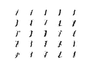
分类控制代码设置为 1 时由 InfoGAN 模型生成的 25 幅图像图
用不同的数字进行实验,并查看图像的确切控制值。
例如,在这种情况下将该值设置为 5(数字= 5)会生成看起来像数字“ 8 ”的图像。
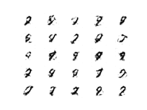
分类控制代码设置为 5 的 InfoGAN 模型生成的 25 幅图像的图
扩展ˌ扩张
本节列出了一些您可能希望探索的扩展教程的想法。
- 改变基数。更新示例以使用分类控制变量的不同基数(例如,更多或更少的值),并查看对训练过程和对生成图像的控制的影响。
- 统一控制变量。更新示例,向辅助模型添加两个统一的连续控制变量,并检查对训练过程的影响和对生成图像的控制。
- 高斯控制变量。更新示例,向辅助模型添加两个高斯连续控制变量,并查看对训练过程的影响和对生成图像的控制。
如果你探索这些扩展,我很想知道。
在下面的评论中发表你的发现。
进一步阅读
如果您想更深入地了解这个主题,本节将提供更多资源。
报纸
- InfoGAN:通过信息最大化生成对抗网络进行可解释表征学习,2016。
- 了解互信息及其在 InfoGAN 中的使用,2016。
- 即时消息算法:信息最大化的变分方法,2004。
应用程序接口
- 硬数据集 API .
- Keras 顺序模型 API
- Keras 卷积层应用编程接口
- 如何“冻结”Keras 层?
- MatplotLib API
- NumPy 随机采样(numpy.random) API
- NumPy 数组操作例程
项目
- InfoGAN(官方),OpenAI,GitHub 。
- 一次性插入:一次性执行插入,GitHub 。
- Keras-GAN:生成对抗网络的 Keras 实现,GitHub 。
- 高级-深度-与-Keras 学习,PacktPublishing,GitHub 。
- 深度学习实现:实现最近的深度学习论文,GitHub 。
文章
- 互信息,维基百科。
- 条件互信息,维基百科。
- InfoGAN:利用互信息上的变分界(两次),2016。
- GANs,互信息,可能还有算法选择?,2016 年。
- 实现 InfoGAN:比看起来容易?,2016 年。
- 成本函数问题,深度学习实现项目,GitHub 。
摘要
在本教程中,您发现了如何从零开始实现信息最大化生成对抗网络模型。
具体来说,您了解到:
- InfoGAN 的动机是希望解开和控制生成图像中的属性。
- InfoGAN 包括添加控制变量,以生成预测控制变量的辅助模型,该模型通过相互信息损失函数进行训练。
- 如何从零开始开发和训练一个 InfoGAN 模型,并使用控制变量来控制模型生成哪个数字。
你有什么问题吗?
在下面的评论中提问,我会尽力回答。

助力广东及东莞地区开发者,代码托管、在线学习与竞赛、技术交流与分享、资源共享、职业发展,成为松山湖开发者首选的工作与学习平台
更多推荐


 29
29 0
0- 0


 已为社区贡献3条内容

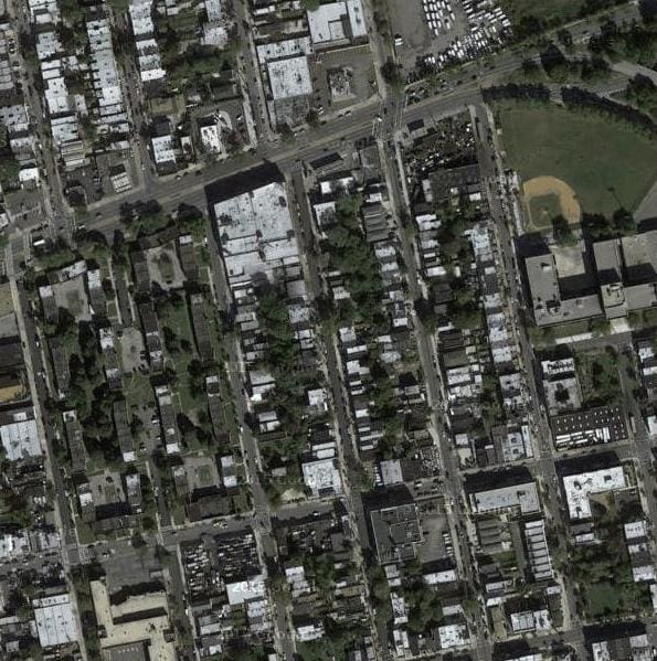
所有评论(0)