前言

        在数字图像处理中，完成图像分割后，我们得到了目标区域和边界，但这些原始像素集合难以直接用于后续的分析、识别和分类。第 11 章的表示与描述正是解决这个问题的核心 —— 通过特定的方法将分割后的区域 / 边界用简洁、有意义的形式表示，并提取能反映其本质特征的描述子，让计算机能够 "理解" 图像中目标的形状、结构和属性。

        本文将结合完整可运行的 Python 代码，详细讲解数字图像处理中表示与描述的核心知识点，所有案例均附带效果对比图，帮助你直观理解每个概念的实际应用。

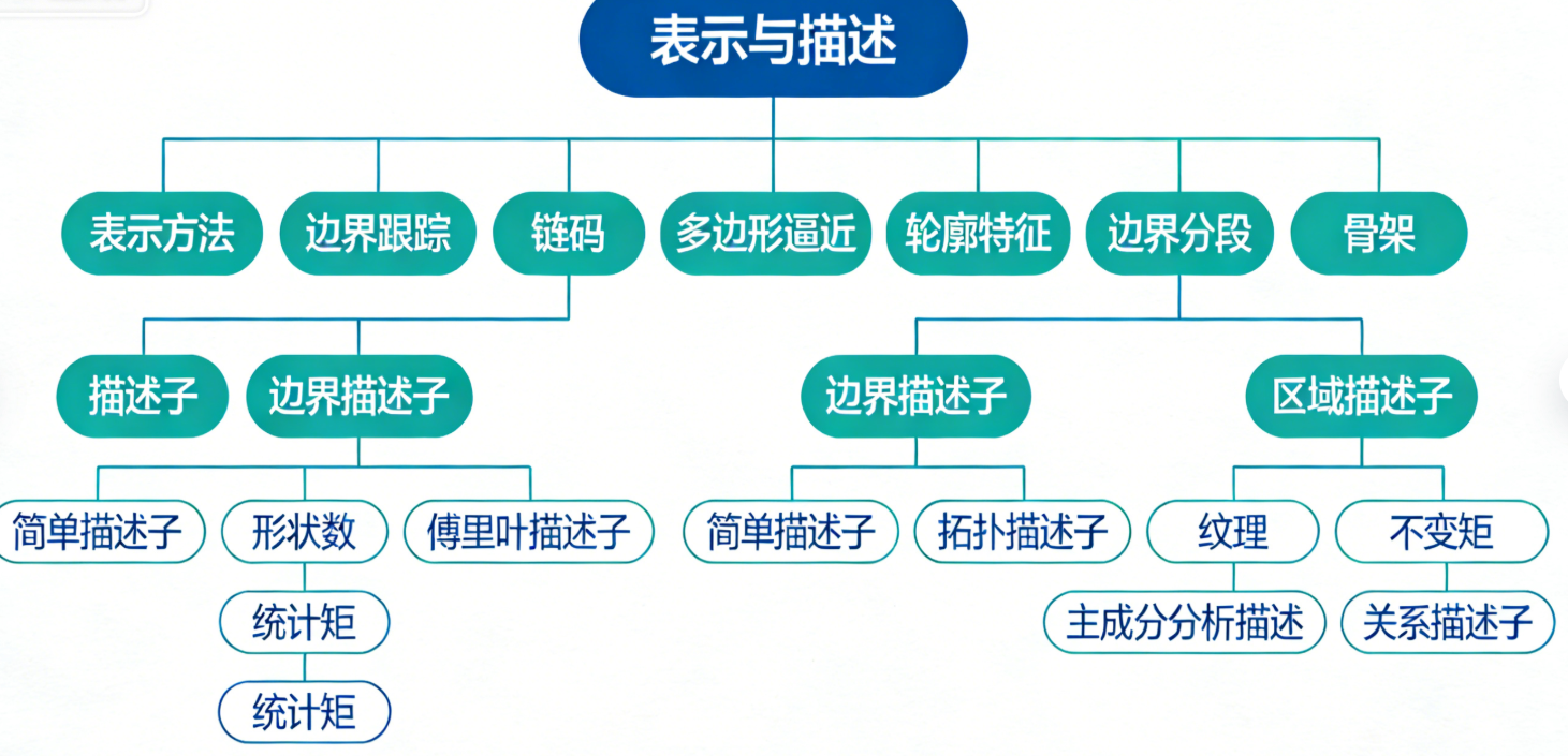
11.1 表示方法

        表示方法的核心是将图像中目标的边界 / 区域从原始像素形式转换为更简洁、易处理的形式，为后续描述做准备。

11.1.1 边界跟踪

        边界跟踪（也叫轮廓提取）是从二值图像中找到目标物体边界像素的过程，OpenCV 中提供了findContours函数实现该功能。

完整代码（边界跟踪）

import cv2
import numpy as np
import matplotlib.pyplot as plt

# 设置matplotlib支持中文显示
plt.rcParams['font.sans-serif'] = ['SimHei']  # 黑体
plt.rcParams['axes.unicode_minus'] = False    # 解决负号显示问题

def boundary_tracking_demo():
    """边界跟踪（轮廓提取）演示"""
    # 1. 读取图像并预处理
    # 读取彩色图像
    img = cv2.imread('test_shape.jpg')
    if img is None:
        print("请确保test_shape.jpg文件存在于当前目录！")
        return
    img_rgb = cv2.cvtColor(img, cv2.COLOR_BGR2RGB)  # 转换为RGB格式（适配matplotlib）
    
    # 灰度化+二值化（分割基础）
    gray = cv2.cvtColor(img, cv2.COLOR_BGR2GRAY)
    ret, binary = cv2.threshold(gray, 127, 255, cv2.THRESH_BINARY_INV)  # 二值化（反相）
    
    # 2. 边界跟踪（查找轮廓）
    contours, hierarchy = cv2.findContours(binary, cv2.RETR_EXTERNAL, cv2.CHAIN_APPROX_SIMPLE)
    
    # 3. 绘制轮廓
    img_contour = img_rgb.copy()
    cv2.drawContours(img_contour, contours, -1, (255, 0, 0), 2)  # 蓝色绘制轮廓
    
    # 4. 效果对比显示
    plt.figure(figsize=(12, 6))
    
    # 原始彩色图
    plt.subplot(1, 3, 1)
    plt.imshow(img_rgb)
    plt.title('原始彩色图像')
    plt.axis('off')
    
    # 二值化图像
    plt.subplot(1, 3, 2)
    plt.imshow(binary, cmap='gray')
    plt.title('二值化图像')
    plt.axis('off')
    
    # 轮廓跟踪结果
    plt.subplot(1, 3, 3)
    plt.imshow(img_contour)
    plt.title('边界跟踪（轮廓提取）结果')
    plt.axis('off')
    
    plt.tight_layout()
    plt.show()

# 运行演示
if __name__ == "__main__":
    boundary_tracking_demo()

代码说明

1. 预处理：先将彩色图转灰度，再二值化（分割出目标区域）；
2. 边界跟踪核心：cv2.findContours是 OpenCV 的核心轮廓提取函数，RETR_EXTERNAL表示只提取最外层轮廓，CHAIN_APPROX_SIMPLE用于压缩轮廓点（减少冗余）；
3. 可视化：将原始图、二值图、轮廓结果放在同一窗口对比，直观展示效果。

11.1.2 链码

        链码（Freeman 链码）是用方向码表示边界点序列的方法，核心是用数字（如 0-7 表示 8 个方向）描述边界的走向，能极大压缩边界数据。

完整代码（链码生成与还原）

import cv2
import numpy as np
import matplotlib.pyplot as plt

plt.rcParams['font.sans-serif'] = ['SimHei']
plt.rcParams['axes.unicode_minus'] = False

# 定义8方向Freeman链码的方向向量（上、右上、右、右下、下、左下、左、左上）
DIRECTIONS = [(-1, 0), (-1, 1), (0, 1), (1, 1), 
              (1, 0), (1, -1), (0, -1), (-1, -1)]

def get_freeman_chaincode(contour):
    """计算轮廓的Freeman链码（8方向）"""
    chaincode = []
    # 取轮廓的第一个点作为起始点
    prev_point = contour[0][0]
    
    for i in range(1, len(contour)):
        curr_point = contour[i][0]
        # 计算当前点相对于前一个点的偏移
        dx = curr_point[0] - prev_point[0]
        dy = curr_point[1] - prev_point[1]
        
        # 查找对应的方向码
        for idx, (dy_dir, dx_dir) in enumerate(DIRECTIONS):
            if dx == dx_dir and dy == dy_dir:
                chaincode.append(idx)
                break
        
        prev_point = curr_point
    
    return chaincode

def chaincode_demo():
    """链码演示"""
    # 1. 读取并预处理图像
    img = cv2.imread('test_shape.jpg')
    if img is None:
        print("请确保test_shape.jpg文件存在于当前目录！")
        return
    img_rgb = cv2.cvtColor(img, cv2.COLOR_BGR2RGB)
    gray = cv2.cvtColor(img, cv2.COLOR_BGR2GRAY)
    ret, binary = cv2.threshold(gray, 127, 255, cv2.THRESH_BINARY_INV)
    
    # 2. 提取轮廓
    contours, _ = cv2.findContours(binary, cv2.RETR_EXTERNAL, cv2.CHAIN_APPROX_NONE)
    # 取最大的轮廓（假设只有一个目标）
    contour = max(contours, key=len)
    
    # 3. 计算链码
    chaincode = get_freeman_chaincode(contour)
    
    # 4. 从链码还原轮廓
    start_point = contour[0][0]
    restored_contour = [start_point]
    current_point = start_point
    
    for code in chaincode:
        dy, dx = DIRECTIONS[code]
        new_point = (current_point[0] + dx, current_point[1] + dy)
        restored_contour.append(new_point)
        current_point = new_point
    
    # 转换为OpenCV轮廓格式
    restored_contour = np.array(restored_contour, dtype=np.int32).reshape(-1, 1, 2)
    
    # 5. 绘制结果
    img_chaincode = img_rgb.copy()
    cv2.drawContours(img_chaincode, [restored_contour], -1, (0, 255, 0), 2)  # 绿色绘制还原的轮廓
    
    # 6. 效果对比
    plt.figure(figsize=(12, 6))
    
    plt.subplot(1, 2, 1)
    plt.imshow(img_rgb)
    plt.title(f'原始图像（链码长度：{len(chaincode)}）')
    plt.axis('off')
    
    plt.subplot(1, 2, 2)
    plt.imshow(img_chaincode)
    plt.title('链码还原的轮廓')
    plt.axis('off')
    
    print(f"Freeman链码（前20个）：{chaincode[:20]}...")
    plt.tight_layout()
    plt.show()

if __name__ == "__main__":
    chaincode_demo()

代码说明

1. 方向定义：8 方向链码对应 8 个偏移向量，覆盖所有相邻像素的方向；
2. 链码计算：遍历轮廓点，计算相邻点的偏移，匹配对应的方向码；
3. 轮廓还原：从起始点出发，根据链码的方向逐步还原轮廓，验证链码的有效性；
4. 优势：链码用少量数字表示完整边界，数据量远小于原始轮廓点。

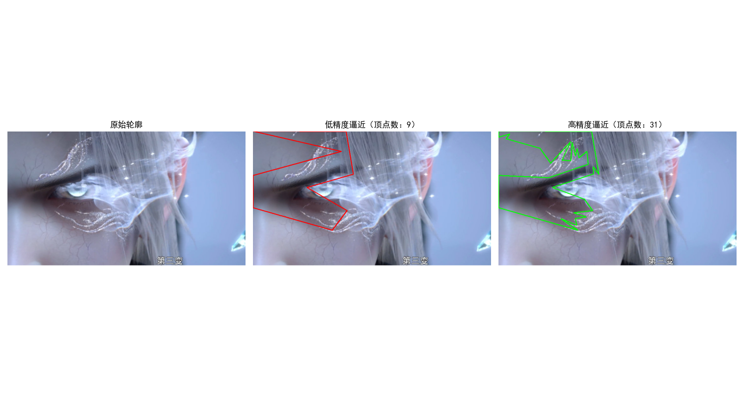
11.1.3 基于最小周长多边形的多边形逼近

        多边形逼近是用简单的多边形拟合复杂边界，最小周长多边形（MPP）是其中经典方法，核心是用尽可能少的边逼近边界，同时保证周长最小。

完整代码（多边形逼近）

import cv2
import numpy as np
import matplotlib.pyplot as plt

plt.rcParams['font.sans-serif'] = ['SimHei']
plt.rcParams['axes.unicode_minus'] = False

def polygon_approximation_demo():
    """基于最小周长思想的多边形逼近演示"""
    # 1. 读取并预处理图像
    img = cv2.imread('test_shape.jpg')
    if img is None:
        print("请确保test_shape.jpg文件存在于当前目录！")
        return
    img_rgb = cv2.cvtColor(img, cv2.COLOR_BGR2RGB)
    gray = cv2.cvtColor(img, cv2.COLOR_BGR2GRAY)
    ret, binary = cv2.threshold(gray, 127, 255, cv2.THRESH_BINARY_INV)
    
    # 2. 提取轮廓
    contours, _ = cv2.findContours(binary, cv2.RETR_EXTERNAL, cv2.CHAIN_APPROX_SIMPLE)
    contour = max(contours, key=len)
    
    # 3. 多边形逼近（Douglas-Peucker算法，近似MPP思想）
    # 计算轮廓周长
    perimeter = cv2.arcLength(contour, closed=True)
    # 不同精度的逼近（epsilon越小，逼近越精细）
    epsilon1 = 0.02 * perimeter  # 低精度（少边）
    epsilon2 = 0.005 * perimeter # 高精度（多边）
    approx1 = cv2.approxPolyDP(contour, epsilon1, closed=True)
    approx2 = cv2.approxPolyDP(contour, epsilon2, closed=True)
    
    # 4. 绘制结果
    img_approx1 = img_rgb.copy()
    img_approx2 = img_rgb.copy()
    cv2.drawContours(img_approx1, [approx1], -1, (255, 0, 0), 2)  # 蓝色：低精度
    cv2.drawContours(img_approx2, [approx2], -1, (0, 255, 0), 2)  # 绿色：高精度
    
    # 5. 效果对比
    plt.figure(figsize=(15, 5))
    
    plt.subplot(1, 3, 1)
    plt.imshow(img_rgb)
    plt.title('原始轮廓')
    plt.axis('off')
    
    plt.subplot(1, 3, 2)
    plt.imshow(img_approx1)
    plt.title(f'低精度逼近（顶点数：{len(approx1)}）')
    plt.axis('off')
    
    plt.subplot(1, 3, 3)
    plt.imshow(img_approx2)
    plt.title(f'高精度逼近（顶点数：{len(approx2)}）')
    plt.axis('off')
    
    plt.tight_layout()
    plt.show()

if __name__ == "__main__":
    polygon_approximation_demo()

代码说明

1. 核心函数：cv2.approxPolyDP是 OpenCV 实现的 Douglas-Peucker 算法，是 MPP 的近似实现；
2. 精度控制：epsilon参数（通常为周长的百分比）决定逼近精度，值越小，多边形越接近原始轮廓；
3. 应用场景：用少量多边形顶点替代大量轮廓点，降低后续计算复杂度。

11.1.4 其他多边形逼近方法（简要实现）

        除了 MPP，常用的还有基于点集拟合、分治的逼近方法，这里实现简单的基于距离阈值的逼近：

import cv2
import numpy as np
import matplotlib.pyplot as plt

plt.rcParams['font.sans-serif'] = ['SimHei']
plt.rcParams['axes.unicode_minus'] = False

def distance_based_approximation(contour, threshold):
    """基于距离阈值的多边形逼近"""
    if len(contour) < 3:
        return contour
    
    approx = [contour[0][0]]  # 起始点
    prev_point = contour[0][0]
    
    for point in contour[1:]:
        curr_point = point[0]
        # 计算欧氏距离
        dist = np.linalg.norm(curr_point - prev_point)
        if dist > threshold:
            approx.append(curr_point)
            prev_point = curr_point
    
    # 闭合轮廓
    approx.append(contour[0][0])
    return np.array(approx, dtype=np.int32).reshape(-1, 1, 2)

def other_polygon_approx_demo():
    """其他多边形逼近方法演示"""
    # 1. 读取并预处理
    img = cv2.imread('test_shape.jpg')
    if img is None:
        print("请确保test_shape.jpg文件存在于当前目录！")
        return
    img_rgb = cv2.cvtColor(img, cv2.COLOR_BGR2RGB)
    gray = cv2.cvtColor(img, cv2.COLOR_BGR2GRAY)
    ret, binary = cv2.threshold(gray, 127, 255, cv2.THRESH_BINARY_INV)
    
    # 2. 提取轮廓
    contours, _ = cv2.findContours(binary, cv2.RETR_EXTERNAL, cv2.CHAIN_APPROX_SIMPLE)
    contour = max(contours, key=len)
    
    # 3. 不同阈值的距离逼近
    approx_low = distance_based_approximation(contour, 10)
    approx_high = distance_based_approximation(contour, 5)
    
    # 4. 绘制
    img_low = img_rgb.copy()
    img_high = img_rgb.copy()
    cv2.drawContours(img_low, [approx_low], -1, (255, 0, 0), 2)
    cv2.drawContours(img_high, [approx_high], -1, (0, 255, 0), 2)
    
    # 5. 对比显示
    plt.figure(figsize=(12, 6))
    
    plt.subplot(1, 2, 1)
    plt.imshow(img_low)
    plt.title('距离阈值10的逼近')
    plt.axis('off')
    
    plt.subplot(1, 2, 2)
    plt.imshow(img_high)
    plt.title('距离阈值5的逼近')
    plt.axis('off')
    
    plt.tight_layout()
    plt.show()

if __name__ == "__main__":
    other_polygon_approx_demo()

11.1.5 轮廓特征

        轮廓特征是描述轮廓几何属性的基础指标，如面积、周长、外接矩形、凸包等。

完整代码（轮廓特征提取）

import cv2
import numpy as np
import matplotlib.pyplot as plt

plt.rcParams['font.sans-serif'] = ['SimHei']
plt.rcParams['axes.unicode_minus'] = False

def contour_features_demo():
    """轮廓特征提取演示"""
    # 1. 读取并预处理
    img = cv2.imread('test_shape.jpg')
    if img is None:
        print("请确保test_shape.jpg文件存在于当前目录！")
        return
    img_rgb = cv2.cvtColor(img, cv2.COLOR_BGR2RGB)
    gray = cv2.cvtColor(img, cv2.COLOR_BGR2GRAY)
    ret, binary = cv2.threshold(gray, 127, 255, cv2.THRESH_BINARY_INV)
    
    # 2. 提取轮廓
    contours, _ = cv2.findContours(binary, cv2.RETR_EXTERNAL, cv2.CHAIN_APPROX_SIMPLE)
    contour = max(contours, key=len)
    
    # 3. 计算轮廓特征
    area = cv2.contourArea(contour)  # 面积
    perimeter = cv2.arcLength(contour, closed=True)  # 周长
    rect = cv2.boundingRect(contour)  # 外接矩形 (x,y,w,h)
    x, y, w, h = rect
    convex_hull = cv2.convexHull(contour)  # 凸包
    aspect_ratio = float(w) / h  # 长宽比
    extent = area / (w * h)  # 延展度（轮廓面积/外接矩形面积）
    
    # 4. 绘制特征
    img_features = img_rgb.copy()
    # 绘制外接矩形
    cv2.rectangle(img_features, (x, y), (x+w, y+h), (255, 0, 0), 2)
    # 绘制凸包
    cv2.drawContours(img_features, [convex_hull], -1, (0, 255, 0), 2)
    
    # 5. 显示结果
    plt.figure(figsize=(10, 6))
    plt.imshow(img_features)
    plt.title(f'轮廓特征：面积={area:.0f}, 周长={perimeter:.0f}, 长宽比={aspect_ratio:.2f}')
    plt.axis('off')
    plt.show()
    
    # 打印详细特征
    print("=== 轮廓特征详细信息 ===")
    print(f"轮廓面积：{area:.2f} 像素")
    print(f"轮廓周长：{perimeter:.2f} 像素")
    print(f"外接矩形：x={x}, y={y}, 宽={w}, 高={h}")
    print(f"长宽比：{aspect_ratio:.2f}")
    print(f"延展度：{extent:.2f}")

if __name__ == "__main__":
    contour_features_demo()

11.1.6 边界分段

        边界分段是将长边界拆分为多个有意义的子段（如角点、直线段），便于局部特征分析。

完整代码（边界分段）

import cv2
import numpy as np
import matplotlib.pyplot as plt

# 设置matplotlib支持中文显示
plt.rcParams['font.sans-serif'] = ['SimHei']
plt.rcParams['axes.unicode_minus'] = False


def boundary_segmentation_demo():
    """边界分段演示（基于角点检测）- 修复版"""
    # 1. 读取并预处理
    img_path = '../picture/GaoDa.png'
    img = cv2.imread(img_path)
    if img is None:
        print(f"错误：未找到图像文件，请检查路径是否正确！路径：{img_path}")
        return

    img_rgb = cv2.cvtColor(img, cv2.COLOR_BGR2RGB)
    gray = cv2.cvtColor(img, cv2.COLOR_BGR2GRAY)

    # 优化：自适应二值化（替代固定阈值127，适配不同亮度的图像）
    # 如果自适应效果差，可改用：ret, binary = cv2.threshold(gray, 0, 255, cv2.THRESH_BINARY_INV + cv2.THRESH_OTSU)
    binary = cv2.adaptiveThreshold(
        gray, 255,
        cv2.ADAPTIVE_THRESH_GAUSSIAN_C,
        cv2.THRESH_BINARY_INV,
        blockSize=11, C=2
    )

    # 2. 提取轮廓（增加轮廓有效性判断）
    contours, _ = cv2.findContours(binary, cv2.RETR_EXTERNAL, cv2.CHAIN_APPROX_SIMPLE)
    if len(contours) == 0:
        print("错误：未检测到任何轮廓，请检查二值化效果！")
        # 显示二值化结果，帮助排查
        plt.figure(figsize=(10, 6))
        plt.imshow(binary, cmap='gray')
        plt.title('二值化结果（无轮廓）')
        plt.axis('off')
        plt.show()
        return
    contour = max(contours, key=len)

    # 检查轮廓点数量
    if len(contour) < 10:  # 轮廓点过少，无法检测角点
        print(f"警告：轮廓点数量过少（仅{len(contour)}个），无法检测角点！")
        return

    # 3. 角点检测（优化参数，增加容错）
    contour_points = contour.reshape(-1, 2).astype(np.float32)
    # 优化参数：降低qualityLevel、减小minDistance，增加maxCorners
    corners = cv2.goodFeaturesToTrack(
        contour_points,
        maxCorners=20,  # 最多检测20个角点
        qualityLevel=0.001,  # 角点质量阈值（降低更易检测）
        minDistance=3  # 角点最小间距（减小更易检测）
    )

    # 4. 容错处理：无角点时的提示
    if corners is None:
        print("提示：未检测到任何角点，已仅绘制轮廓！")
        img_segment = img_rgb.copy()
        cv2.drawContours(img_segment, [contour], -1, (0, 0, 255), 1)
        plt.figure(figsize=(10, 6))
        plt.imshow(img_segment)
        plt.title('边界分段（未检测到角点）')
        plt.axis('off')
        plt.show()
        return

    # 修复：替换弃用的np.int0为np.intp
    corners = np.intp(corners)

    # 5. 绘制分段结果
    img_segment = img_rgb.copy()
    # 绘制原始轮廓
    cv2.drawContours(img_segment, [contour], -1, (0, 0, 255), 1)
    # 绘制角点（分段点）
    for corner in corners:
        x, y = corner.ravel()
        cv2.circle(img_segment, (x, y), 3, (255, 0, 0), -1)  # 蓝色角点

    # 6. 显示结果
    plt.figure(figsize=(10, 6))
    plt.imshow(img_segment)
    plt.title(f'边界分段（检测到{len(corners)}个角点/分段点）')
    plt.axis('off')
    plt.show()


if __name__ == "__main__":
    boundary_segmentation_demo()

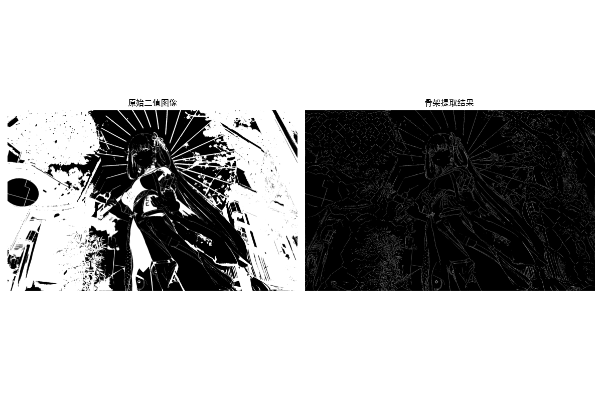
11.1.7 骨架

        骨架（细化）是将区域收缩为单像素宽度的中心线，保留区域的拓扑结构，常用于字符识别、指纹识别等。

完整代码（骨架提取）

import cv2
import numpy as np
import matplotlib.pyplot as plt

plt.rcParams['font.sans-serif'] = ['SimHei']
plt.rcParams['axes.unicode_minus'] = False

def skeletonize(image):
    """骨架提取（细化）"""
    # 转换为二值图（确保背景为0，前景为255）
    size = np.size(image)
    skel = np.zeros(image.shape, np.uint8)
    
    ret, img = cv2.threshold(image, 127, 255, 0)
    element = cv2.getStructuringElement(cv2.MORPH_CROSS, (3, 3))
    done = False
    
    while not done:
        # 腐蚀
        eroded = cv2.erode(img, element)
        # 开运算
        temp = cv2.dilate(eroded, element)
        temp = cv2.subtract(img, temp)
        skel = cv2.bitwise_or(skel, temp)
        img = eroded.copy()
        
        # 判断是否所有像素都为0
        zeros = size - cv2.countNonZero(img)
        if zeros == size:
            done = True
    
    return skel

def skeleton_demo():
    """骨架提取演示"""
    # 1. 读取并预处理
    img = cv2.imread('test_shape.jpg')
    if img is None:
        print("请确保test_shape.jpg文件存在于当前目录！")
        return
    img_rgb = cv2.cvtColor(img, cv2.COLOR_BGR2RGB)
    gray = cv2.cvtColor(img, cv2.COLOR_BGR2GRAY)
    ret, binary = cv2.threshold(gray, 127, 255, cv2.THRESH_BINARY_INV)
    
    # 2. 提取骨架
    skel = skeletonize(binary)
    
    # 3. 效果对比
    plt.figure(figsize=(12, 6))
    
    plt.subplot(1, 2, 1)
    plt.imshow(binary, cmap='gray')
    plt.title('原始二值图像')
    plt.axis('off')
    
    plt.subplot(1, 2, 2)
    plt.imshow(skel, cmap='gray')
    plt.title('骨架提取结果')
    plt.axis('off')
    
    plt.tight_layout()
    plt.show()

if __name__ == "__main__":
    skeleton_demo()

11.2 边界描述子

        边界描述子是从边界表示中提取的定量特征，用于区分不同形状的边界，核心是平移、旋转、尺度不变性（尽可能）。

11.2.1 简单描述子

        简单边界描述子包括：边界长度、直径、矩形度、曲率等，是最基础的描述子。

完整代码（简单边界描述子）

import cv2
import numpy as np
import matplotlib.pyplot as plt

# 设置matplotlib支持中文显示
plt.rcParams['font.sans-serif'] = ['SimHei']
plt.rcParams['axes.unicode_minus'] = False


def simple_boundary_descriptors_demo():
    """简单边界描述子演示（优化修复版）"""
    # 1. 读取并预处理
    img_path = '../picture/KanTeLeiLa.png'
    img = cv2.imread(img_path)
    if img is None:
        print(f"错误：未找到图像文件，请检查路径是否正确！路径：{img_path}")
        return

    img_rgb = cv2.cvtColor(img, cv2.COLOR_BGR2RGB)
    gray = cv2.cvtColor(img, cv2.COLOR_BGR2GRAY)

    # 优化：替换固定阈值为自适应二值化（适配不同图像）
    # 若效果不佳，可改用大津法：ret, binary = cv2.threshold(gray, 0, 255, cv2.THRESH_BINARY_INV + cv2.THRESH_OTSU)
    binary = cv2.adaptiveThreshold(
        gray, 255,
        cv2.ADAPTIVE_THRESH_GAUSSIAN_C,
        cv2.THRESH_BINARY_INV,
        blockSize=11, C=2
    )

    # 2. 提取轮廓（增加鲁棒性校验）
    contours, _ = cv2.findContours(binary, cv2.RETR_EXTERNAL, cv2.CHAIN_APPROX_SIMPLE)
    if len(contours) == 0:
        print("错误：未检测到任何轮廓，请检查二值化效果！")
        # 显示二值化结果辅助排查
        plt.figure(figsize=(10, 6))
        plt.imshow(binary, cmap='gray')
        plt.title('二值化结果（无轮廓）')
        plt.axis('off')
        plt.show()
        return
    contour = max(contours, key=len)

    # 3. 计算简单描述子
    # 3.1 边界长度（周长）
    length = cv2.arcLength(contour, closed=True)

    # 3.2 边界直径（最远两点距离）- 优化：替换双重循环为向量化计算，提升效率
    contour_points = contour.reshape(-1, 2).astype(np.float32)
    if len(contour_points) < 2:
        diameter = 0
    else:
        # 用scipy的pdist计算成对距离（若未安装scipy，可保留原循环，仅优化校验）
        try:
            from scipy.spatial.distance import pdist
            dists = pdist(contour_points)
            diameter = np.max(dists)
        except ImportError:
            # 备用方案：原循环+提前终止（减少计算量）
            dists = []
            max_dist = 0
            for i in range(len(contour_points)):
                for j in range(i + 1, len(contour_points)):
                    dist = np.linalg.norm(contour_points[i] - contour_points[j])
                    if dist > max_dist:
                        max_dist = dist
            diameter = max_dist

    # 3.3 矩形度（轮廓面积/最小外接矩形面积）
    area = cv2.contourArea(contour)
    rect = cv2.minAreaRect(contour)
    rect_w, rect_h = rect[1]
    rect_area = rect_w * rect_h
    rectangularity = area / rect_area if rect_area > 0 else 0

    # 3.4 圆形度（4π*面积/周长²）- 增加分母非零校验
    circularity = (4 * np.pi * area) / (length ** 2) if (length > 1e-6 and area > 0) else 0

    # 4. 绘制最小外接矩形 - 修复：替换弃用的np.int0为np.intp
    box = cv2.boxPoints(rect)
    box = np.intp(box)  # 核心修复：消除弃用警告
    img_descriptors = img_rgb.copy()
    cv2.drawContours(img_descriptors, [box], 0, (0, 255, 0), 2)
    # 额外：绘制轮廓（便于对比）
    cv2.drawContours(img_descriptors, [contour], -1, (255, 0, 0), 1)

    # 5. 显示结果（增加二值化对比图）
    plt.figure(figsize=(15, 6))

    plt.subplot(1, 2, 1)
    plt.imshow(binary, cmap='gray')
    plt.title('二值化图像')
    plt.axis('off')

    plt.subplot(1, 2, 2)
    plt.imshow(img_descriptors)
    plt.title(f'边界描述子可视化\n圆形度={circularity:.2f}, 矩形度={rectangularity:.2f}')
    plt.axis('off')

    plt.tight_layout()
    plt.show()

    # 打印描述子（格式化输出更清晰）
    print("=== 简单边界描述子 ===")
    print(f"边界长度（周长）：{length:.2f} 像素")
    print(f"边界直径（最远点距离）：{diameter:.2f} 像素")
    print(f"轮廓面积：{area:.2f} 像素²")
    print(f"最小外接矩形面积：{rect_area:.2f} 像素²")
    print(f"矩形度（面积/外接矩形面积）：{rectangularity:.2f}")
    print(f"圆形度（4π*面积/周长²）：{circularity:.2f}")


if __name__ == "__main__":
    simple_boundary_descriptors_demo()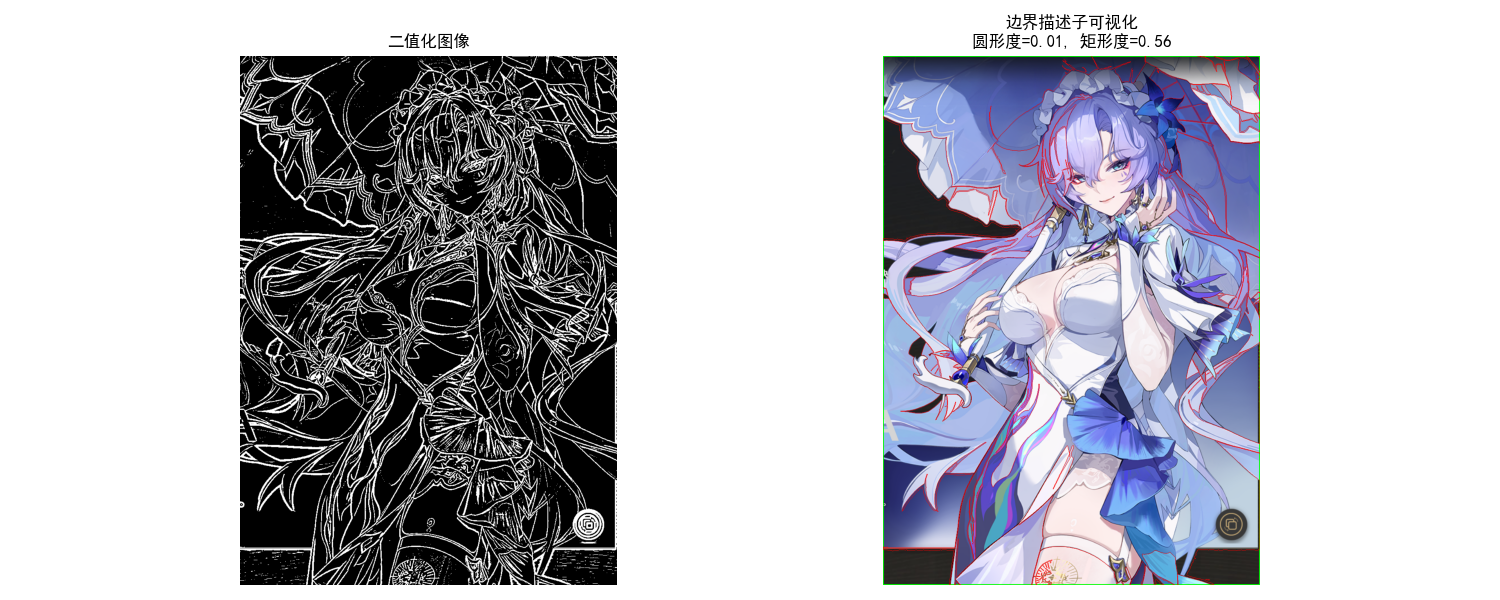

11.2.2 形状数

        形状数是基于链码的归一化描述子，具有平移、旋转不变性，核心是最小差分链码。

完整代码（形状数）

import cv2
import numpy as np
import matplotlib.pyplot as plt

plt.rcParams['font.sans-serif'] = ['SimHei']
plt.rcParams['axes.unicode_minus'] = False

# 8方向链码方向向量
DIRECTIONS = [(-1, 0), (-1, 1), (0, 1), (1, 1), 
              (1, 0), (1, -1), (0, -1), (-1, -1)]

def get_chaincode(contour):
    """获取轮廓的Freeman链码"""
    chaincode = []
    prev_point = contour[0][0]
    for i in range(1, len(contour)):
        curr_point = contour[i][0]
        dx = curr_point[0] - prev_point[0]
        dy = curr_point[1] - prev_point[1]
        for idx, (dy_dir, dx_dir) in enumerate(DIRECTIONS):
            if dx == dx_dir and dy == dy_dir:
                chaincode.append(idx)
                break
        prev_point = curr_point
    return chaincode

def get_shape_number(chaincode):
    """计算形状数（最小差分链码）"""
    # 计算差分链码
    diff_chain = [(chaincode[i] - chaincode[i-1]) % 8 for i in range(1, len(chaincode))]
    diff_chain.append((chaincode[0] - chaincode[-1]) % 8)
    
    # 找到最小循环移位的差分链码（形状数）
    min_diff = diff_chain.copy()
    for i in range(1, len(diff_chain)):
        shifted = diff_chain[i:] + diff_chain[:i]
        if shifted < min_diff:
            min_diff = shifted
    
    return min_diff

def shape_number_demo():
    """形状数演示"""
    # 1. 读取并预处理
    img = cv2.imread('test_shape.jpg')
    if img is None:
        print("请确保test_shape.jpg文件存在于当前目录！")
        return
    img_rgb = cv2.cvtColor(img, cv2.COLOR_BGR2RGB)
    gray = cv2.cvtColor(img, cv2.COLOR_BGR2GRAY)
    ret, binary = cv2.threshold(gray, 127, 255, cv2.THRESH_BINARY_INV)
    
    # 2. 提取轮廓
    contours, _ = cv2.findContours(binary, cv2.RETR_EXTERNAL, cv2.CHAIN_APPROX_NONE)
    contour = max(contours, key=len)
    
    # 3. 计算链码和形状数
    chaincode = get_chaincode(contour)
    shape_number = get_shape_number(chaincode)
    
    # 4. 显示结果
    plt.figure(figsize=(10, 6))
    plt.imshow(img_rgb)
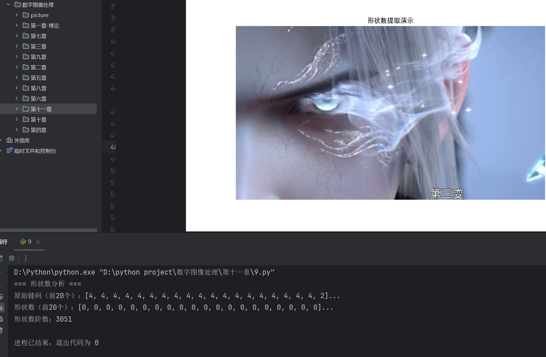
    plt.title('形状数提取演示')
    plt.axis('off')
    plt.show()
    
    # 打印结果
    print("=== 形状数分析 ===")
    print(f"原始链码（前20个）：{chaincode[:20]}...")
    print(f"形状数（前20个）：{shape_number[:20]}...")
    print(f"形状数阶数：{len(shape_number)}")

if __name__ == "__main__":
    shape_number_demo()

11.2.3 傅里叶描述子

        傅里叶描述子（FD）是基于边界点的傅里叶变换提取的描述子，具有平移、旋转、尺度不变性，是最常用的边界描述子之一。

完整代码（傅里叶描述子）

import cv2
import numpy as np
import matplotlib.pyplot as plt

plt.rcParams['font.sans-serif'] = ['SimHei']
plt.rcParams['axes.unicode_minus'] = False

def fourier_descriptors(contour, num_coeffs=10):
    """计算轮廓的傅里叶描述子（归一化，保留前num_coeffs个系数）"""
    # 将轮廓转换为复数序列
    contour_points = contour.reshape(-1, 2)
    z = contour_points[:, 0] + 1j * contour_points[:, 1]
    
    # 傅里叶变换
    f = np.fft.fft(z)
    
    # 归一化（消除平移、旋转、尺度影响）
    # 1. 消除尺度：除以第一个系数的模
    f_normalized = f / np.abs(f[0])
    # 2. 消除旋转：除以第一个系数的相位
    f_normalized = f_normalized / np.exp(1j * np.angle(f_normalized[0]))
    # 3. 只保留前num_coeffs个系数（低频，主要特征）
    fd = f_normalized[:num_coeffs]
    
    return fd, f

def reconstruct_contour(fd, original_length):
    """从傅里叶描述子还原轮廓"""
    # 补零恢复长度
    f_recon = np.zeros(original_length, dtype=np.complex128)
    f_recon[:len(fd)] = fd
    # 共轭对称
    f_recon[-len(fd)+1:] = np.conj(fd[1:][::-1])
    
    # 逆傅里叶变换
    z_recon = np.fft.ifft(f_recon)
    recon_contour = np.column_stack((np.real(z_recon), np.imag(z_recon))).astype(np.int32)
    recon_contour = recon_contour.reshape(-1, 1, 2)
    
    return recon_contour

def fourier_descriptors_demo():
    """傅里叶描述子演示"""
    # 1. 读取并预处理
    img = cv2.imread('test_shape.jpg')
    if img is None:
        print("请确保test_shape.jpg文件存在于当前目录！")
        return
    img_rgb = cv2.cvtColor(img, cv2.COLOR_BGR2RGB)
    gray = cv2.cvtColor(img, cv2.COLOR_BGR2GRAY)
    ret, binary = cv2.threshold(gray, 127, 255, cv2.THRESH_BINARY_INV)
    
    # 2. 提取轮廓
    contours, _ = cv2.findContours(binary, cv2.RETR_EXTERNAL, cv2.CHAIN_APPROX_NONE)
    contour = max(contours, key=len)
    original_length = len(contour)
    
    # 3. 计算傅里叶描述子
    fd, f = fourier_descriptors(contour, num_coeffs=10)
    
    # 4. 从描述子还原轮廓
    recon_contour = reconstruct_contour(fd, original_length)
    
    # 5. 绘制结果
    img_fd = img_rgb.copy()
    cv2.drawContours(img_fd, [recon_contour], -1, (0, 255, 0), 2)
    
    # 6. 效果对比
    plt.figure(figsize=(12, 6))
    
    plt.subplot(1, 2, 1)
    plt.imshow(img_rgb)
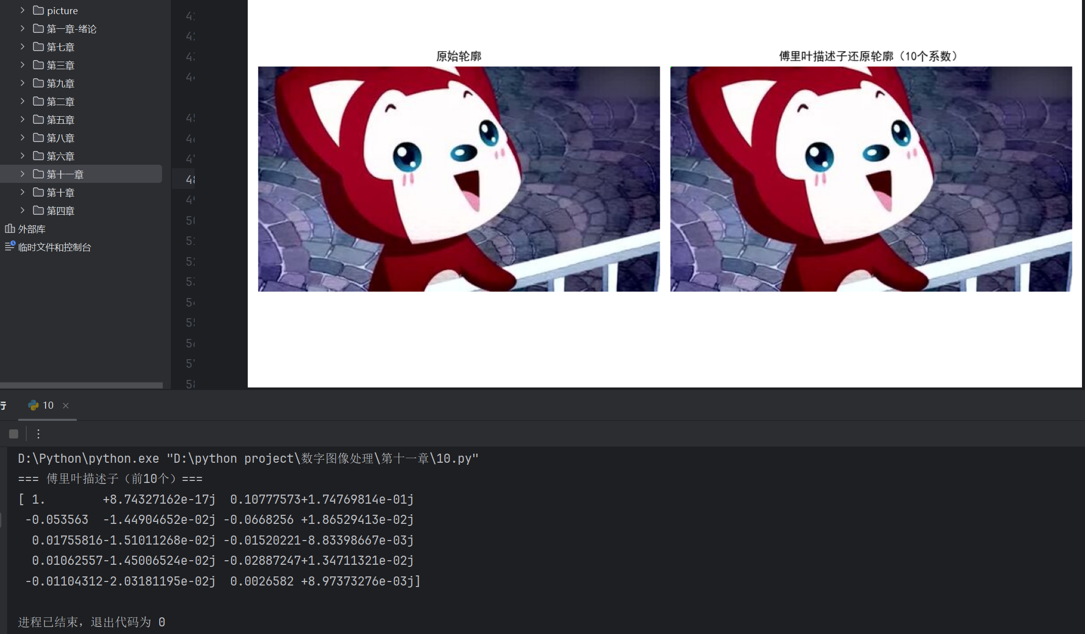
    plt.title('原始轮廓')
    plt.axis('off')
    
    plt.subplot(1, 2, 2)
    plt.imshow(img_fd)
    plt.title('傅里叶描述子还原轮廓（10个系数）')
    plt.axis('off')
    
    plt.tight_layout()
    plt.show()
    
    # 打印傅里叶描述子
    print("=== 傅里叶描述子（前10个）===")
    print(fd)

if __name__ == "__main__":
    fourier_descriptors_demo()

11.2.4 统计矩

        统计矩（如均值、方差、偏度、峰度）可用于描述边界点的分布特征，是简单有效的统计型描述子。

完整代码（统计矩）

import cv2
import numpy as np
import scipy.stats as stats
import matplotlib.pyplot as plt

plt.rcParams['font.sans-serif'] = ['SimHei']
plt.rcParams['axes.unicode_minus'] = False

def statistical_moments_demo():
    """边界的统计矩描述子演示"""
    # 1. 读取并预处理
    img = cv2.imread('test_shape.jpg')
    if img is None:
        print("请确保test_shape.jpg文件存在于当前目录！")
        return
    img_rgb = cv2.cvtColor(img, cv2.COLOR_BGR2RGB)
    gray = cv2.cvtColor(img, cv2.COLOR_BGR2GRAY)
    ret, binary = cv2.threshold(gray, 127, 255, cv2.THRESH_BINARY_INV)
    
    # 2. 提取轮廓
    contours, _ = cv2.findContours(binary, cv2.RETR_EXTERNAL, cv2.CHAIN_APPROX_SIMPLE)
    contour = max(contours, key=len)
    contour_points = contour.reshape(-1, 2)
    
    # 3. 计算统计矩
    # 分离x、y坐标
    x = contour_points[:, 0]
    y = contour_points[:, 1]
    
    # 一阶矩（均值）
    mean_x = np.mean(x)
    mean_y = np.mean(y)
    
    # 二阶矩（方差）
    var_x = np.var(x)
    var_y = np.var(y)
    
    # 三阶矩（偏度）
    skew_x = stats.skew(x)
    skew_y = stats.skew(y)
    
    # 四阶矩（峰度）
    kurt_x = stats.kurtosis(x)
    kurt_y = stats.kurtosis(y)
    
    # 4. 绘制均值点
    img_moments = img_rgb.copy()
    cv2.circle(img_moments, (int(mean_x), int(mean_y)), 5, (255, 0, 0), -1)
    
    # 5. 显示结果
    plt.figure(figsize=(10, 6))
    plt.imshow(img_moments)
    plt.title(f'边界点均值位置（红色点）：({mean_x:.1f}, {mean_y:.1f})')
    plt.axis('off')
    plt.show()
    
    # 打印统计矩
    print("=== 边界点统计矩 ===")
    print(f"X坐标 - 均值：{mean_x:.2f}, 方差：{var_x:.2f}, 偏度：{skew_x:.2f}, 峰度：{kurt_x:.2f}")
    print(f"Y坐标 - 均值：{mean_y:.2f}, 方差：{var_y:.2f}, 偏度：{skew_y:.2f}, 峰度：{kurt_y:.2f}")

if __name__ == "__main__":
    statistical_moments_demo()

11.3 区域描述子

        区域描述子直接从目标区域（而非边界）提取特征，更全面地反映目标的属性。

11.3.1 简单描述子

        区域简单描述子包括：面积、重心、灰度均值、纹理均值等，是区域最基础的特征。

完整代码（区域简单描述子）

import cv2
import numpy as np
import matplotlib.pyplot as plt

plt.rcParams['font.sans-serif'] = ['SimHei']
plt.rcParams['axes.unicode_minus'] = False

def simple_region_descriptors_demo():
    """区域简单描述子演示"""
    # 1. 读取图像
    img = cv2.imread('test_shape.jpg')
    if img is None:
        print("请确保test_shape.jpg文件存在于当前目录！")
        return
    img_rgb = cv2.cvtColor(img, cv2.COLOR_BGR2RGB)
    gray = cv2.cvtColor(img, cv2.COLOR_BGR2GRAY)
    
    # 2. 分割区域（二值化）
    ret, binary = cv2.threshold(gray, 127, 255, cv2.THRESH_BINARY_INV)
    # 提取掩码（前景为1，背景为0）
    mask = binary / 255
    
    # 3. 计算区域描述子
    # 1. 区域面积
    area = cv2.countNonZero(binary)
    # 2. 重心
    moments = cv2.moments(binary)
    cx = moments['m10'] / moments['m00'] if moments['m00'] > 0 else 0
    cy = moments['m01'] / moments['m00'] if moments['m00'] > 0 else 0
    # 3. 灰度均值
    mean_gray = np.mean(gray[binary == 255])
    # 4. 灰度标准差
    std_gray = np.std(gray[binary == 255])
    # 5. 填充率（区域面积/外接矩形面积）
    contours, _ = cv2.findContours(binary, cv2.RETR_EXTERNAL, cv2.CHAIN_APPROX_SIMPLE)
    contour = max(contours, key=len)
    x, y, w, h = cv2.boundingRect(contour)
    fill_ratio = area / (w * h) if (w * h) > 0 else 0
    
    # 4. 绘制重心和外接矩形
    img_descriptors = img_rgb.copy()
    cv2.rectangle(img_descriptors, (x, y), (x+w, y+h), (255, 0, 0), 2)
    cv2.circle(img_descriptors, (int(cx), int(cy)), 5, (0, 255, 0), -1)
    
    # 5. 显示结果
    plt.figure(figsize=(10, 6))
    plt.imshow(img_descriptors)
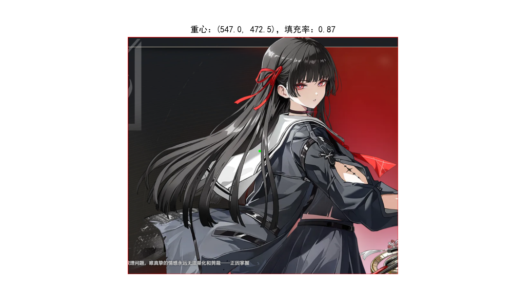
    plt.title(f'重心：({cx:.1f}, {cy:.1f})，填充率：{fill_ratio:.2f}')
    plt.axis('off')
    plt.show()
    
    # 打印描述子
    print("=== 区域简单描述子 ===")
    print(f"区域面积：{area} 像素")
    print(f"重心坐标：({cx:.2f}, {cy:.2f})")
    print(f"区域灰度均值：{mean_gray:.2f}")
    print(f"区域灰度标准差：{std_gray:.2f}")
    print(f"填充率：{fill_ratio:.2f}")

if __name__ == "__main__":
    simple_region_descriptors_demo()

11.3.2 拓扑描述子

        拓扑描述子描述区域的连通性、孔洞数等拓扑属性，具有平移、旋转、尺度不变性。

完整代码（拓扑描述子）

import cv2
import numpy as np
import matplotlib.pyplot as plt

plt.rcParams['font.sans-serif'] = ['SimHei']
plt.rcParams['axes.unicode_minus'] = False

def topological_descriptors_demo():
    """拓扑描述子演示（连通域、孔洞数）"""
    # 1. 读取并预处理（建议使用带孔洞的图像，如圆环）
    img = cv2.imread('test_shape_with_hole.jpg')
    if img is None:
        print("请确保test_shape_with_hole.jpg文件存在于当前目录（建议使用带孔洞的图像）！")
        # 生成一个带孔洞的测试图像
        img = np.zeros((300, 300, 3), dtype=np.uint8)
        cv2.circle(img, (150, 150), 100, (255, 255, 255), -1)
        cv2.circle(img, (150, 150), 50, (0, 0, 0), -1)
        img_rgb = img.copy()
    
    img_rgb = cv2.cvtColor(img, cv2.COLOR_BGR2RGB)
    gray = cv2.cvtColor(img, cv2.COLOR_BGR2GRAY)
    ret, binary = cv2.threshold(gray, 127, 255, cv2.THRESH_BINARY)
    
    # 2. 计算拓扑描述子
    # 1. 连通域数量（使用RETR_CCOMP检索所有轮廓，包括孔洞）
    contours, hierarchy = cv2.findContours(binary, cv2.RETR_CCOMP, cv2.CHAIN_APPROX_SIMPLE)
    
    # 统计连通域和孔洞数
    num_regions = 0  # 连通域数
    num_holes = 0    # 孔洞数
    for i in range(len(hierarchy[0])):
        # hierarchy格式：[Next, Previous, First_Child, Parent]
        if hierarchy[0][i][3] == -1:
            # 没有父节点，是外部轮廓（连通域）
            num_regions += 1
        else:
            # 有父节点，是内部轮廓（孔洞）
            num_holes += 1
    
    # 2. 欧拉数（连通域数 - 孔洞数）
    euler_number = num_regions - num_holes
    
    # 3. 绘制轮廓（外部轮廓红色，孔洞轮廓绿色）
    img_topology = img_rgb.copy()
    for i, cnt in enumerate(contours):
        if hierarchy[0][i][3] == -1:
            cv2.drawContours(img_topology, [cnt], -1, (255, 0, 0), 2)  # 红色：外部轮廓
        else:
            cv2.drawContours(img_topology, [cnt], -1, (0, 255, 0), 2)  # 绿色：孔洞轮廓
    
    # 4. 显示结果
    plt.figure(figsize=(10, 6))
    plt.imshow(img_topology)
    plt.title(f'连通域数：{num_regions}, 孔洞数：{num_holes}, 欧拉数：{euler_number}')
    plt.axis('off')
    plt.show()
    
    # 打印拓扑描述子
    print("=== 拓扑描述子 ===")
    print(f"连通域数量：{num_regions}")
    print(f"孔洞数量：{num_holes}")
    print(f"欧拉数：{euler_number}")

if __name__ == "__main__":
    topological_descriptors_demo()

11.3.3 纹理

        纹理描述子用于描述区域的灰度分布规律，常用的有灰度共生矩阵（GLCM）、LBP 等。

完整代码（纹理描述子）

import cv2
import numpy as np
from skimage.feature import graycomatrix, graycoprops
import matplotlib.pyplot as plt

plt.rcParams['font.sans-serif'] = ['SimHei']
plt.rcParams['axes.unicode_minus'] = False

def texture_descriptors_demo():
    """纹理描述子演示（灰度共生矩阵）"""
    # 1. 读取图像
    img = cv2.imread('test_texture.jpg')
    if img is None:
        print("请确保test_texture.jpg文件存在于当前目录！")
        # 生成测试纹理图像
        img = np.random.randint(0, 255, (300, 300, 3), dtype=np.uint8)
    img_rgb = cv2.cvtColor(img, cv2.COLOR_BGR2RGB)
    gray = cv2.cvtColor(img, cv2.COLOR_BGR2GRAY)
    
    # 2. 计算灰度共生矩阵（GLCM）
    # 参数：图像、距离、角度、灰度级、是否对称、是否归一化
    glcm = graycomatrix(gray, distances=[5], angles=[0, np.pi/4, np.pi/2, 3*np.pi/4],
                        levels=256, symmetric=True, normed=True)
    
    # 3. 提取纹理特征
    contrast = graycoprops(glcm, 'contrast')  # 对比度
    dissimilarity = graycoprops(glcm, 'dissimilarity')  # 相异性
    homogeneity = graycoprops(glcm, 'homogeneity')  # 同质性
    energy = graycoprops(glcm, 'energy')  # 能量
    correlation = graycoprops(glcm, 'correlation')  # 相关性
    
    # 4. 显示结果
    plt.figure(figsize=(12, 8))
    
    plt.subplot(2, 1, 1)
    plt.imshow(img_rgb)
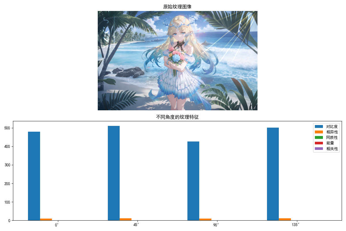
    plt.title('原始纹理图像')
    plt.axis('off')
    
    plt.subplot(2, 1, 2)
    # 绘制不同角度的纹理特征
    angles = ['0°', '45°', '90°', '135°']
    x = np.arange(len(angles))
    width = 0.15
    
    plt.bar(x - 2*width, contrast[0], width, label='对比度')
    plt.bar(x - width, dissimilarity[0], width, label='相异性')
    plt.bar(x, homogeneity[0], width, label='同质性')
    plt.bar(x + width, energy[0], width, label='能量')
    plt.bar(x + 2*width, correlation[0], width, label='相关性')
    
    plt.xticks(x, angles)
    plt.title('不同角度的纹理特征')
    plt.legend()
    plt.tight_layout()
    plt.show()
    
    # 打印纹理特征
    print("=== 纹理描述子（灰度共生矩阵）===")
    print(f"对比度（各角度）：{contrast[0]}")
    print(f"相异性（各角度）：{dissimilarity[0]}")
    print(f"同质性（各角度）：{homogeneity[0]}")
    print(f"能量（各角度）：{energy[0]}")
    print(f"相关性（各角度）：{correlation[0]}")

if __name__ == "__main__":
    texture_descriptors_demo()

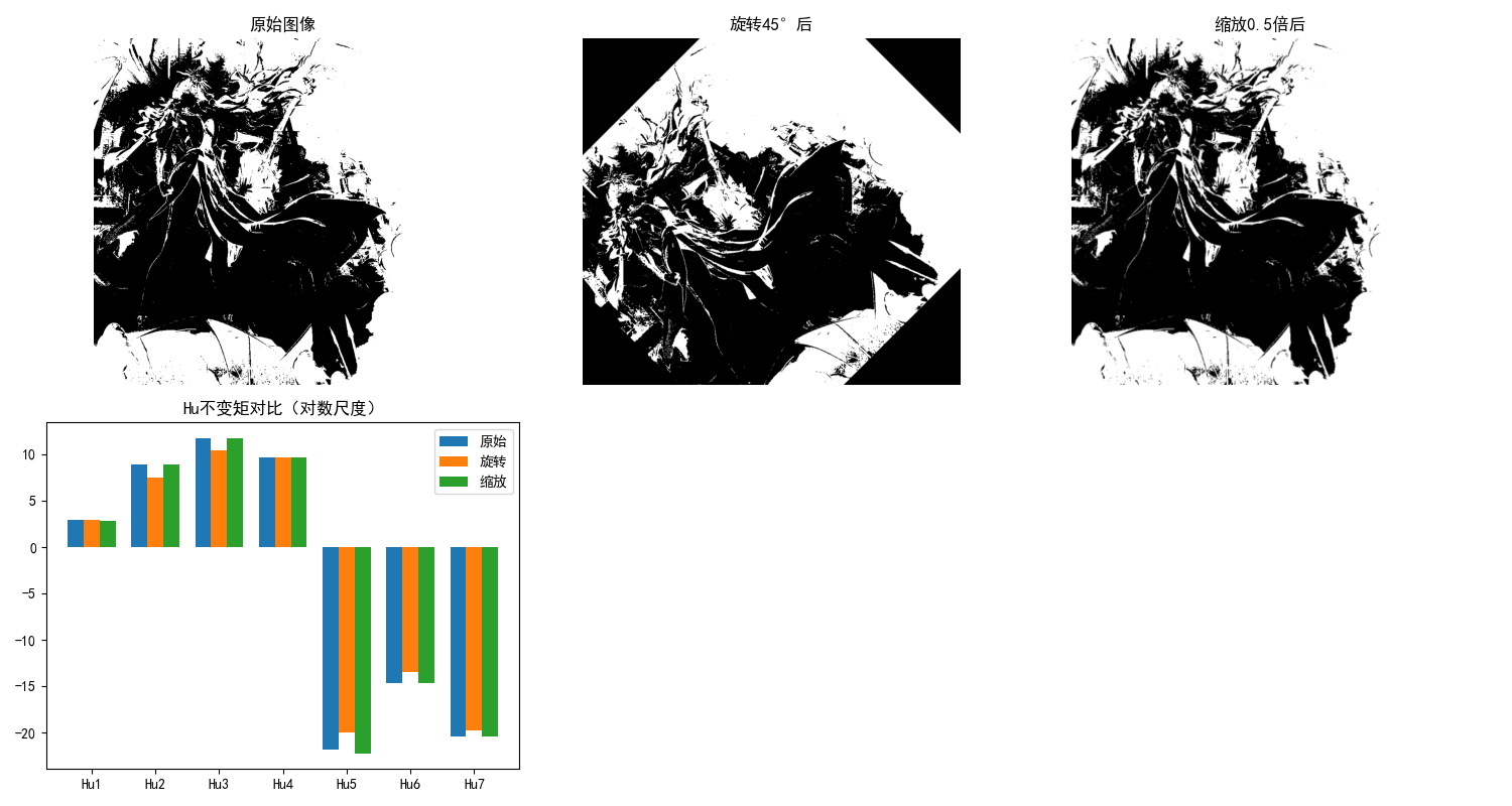
11.3.4 不变矩

        不变矩（Hu 矩）是具有平移、旋转、尺度不变性的区域描述子，是模式识别中经典的特征。

完整代码（不变矩）

import cv2
import numpy as np
import matplotlib.pyplot as plt

plt.rcParams['font.sans-serif'] = ['SimHei']
plt.rcParams['axes.unicode_minus'] = False

def hu_moments_demo():
    """不变矩（Hu矩）演示"""
    # 1. 读取并预处理
    img = cv2.imread('test_shape.jpg')
    if img is None:
        print("请确保test_shape.jpg文件存在于当前目录！")
        return
    img_rgb = cv2.cvtColor(img, cv2.COLOR_BGR2RGB)
    gray = cv2.cvtColor(img, cv2.COLOR_BGR2GRAY)
    ret, binary = cv2.threshold(gray, 127, 255, cv2.THRESH_BINARY_INV)
    
    # 2. 计算Hu不变矩
    moments = cv2.moments(binary)
    hu_moments = cv2.HuMoments(moments)
    # 取对数（便于观察，Hu矩值通常很小）
    hu_moments_log = -np.sign(hu_moments) * np.log10(np.abs(hu_moments))
    
    # 3. 生成变换后的图像（验证不变性）
    # 旋转45度
    rows, cols = binary.shape
    M_rot = cv2.getRotationMatrix2D((cols/2, rows/2), 45, 1)
    binary_rot = cv2.warpAffine(binary, M_rot, (cols, rows))
    # 缩放0.5倍
    M_scale = cv2.resize(binary, (0,0), fx=0.5, fy=0.5)
    binary_scale = cv2.resize(M_scale, (cols, rows))
    
    # 计算变换后的Hu矩
    hu_rot = cv2.HuMoments(cv2.moments(binary_rot))
    hu_rot_log = -np.sign(hu_rot) * np.log10(np.abs(hu_rot))
    hu_scale = cv2.HuMoments(cv2.moments(binary_scale))
    hu_scale_log = -np.sign(hu_scale) * np.log10(np.abs(hu_scale))
    
    # 4. 效果对比
    plt.figure(figsize=(15, 8))
    
    # 原始图像
    plt.subplot(2, 3, 1)
    plt.imshow(binary, cmap='gray')
    plt.title('原始图像')
    plt.axis('off')
    
    # 旋转后图像
    plt.subplot(2, 3, 2)
    plt.imshow(binary_rot, cmap='gray')
    plt.title('旋转45°后')
    plt.axis('off')
    
    # 缩放后图像
    plt.subplot(2, 3, 3)
    plt.imshow(binary_scale, cmap='gray')
    plt.title('缩放0.5倍后')
    plt.axis('off')
    
    # Hu矩对比
    plt.subplot(2, 3, 4)
    moments_idx = [f'Hu{i+1}' for i in range(7)]
    x = np.arange(len(moments_idx))
    width = 0.25
    
    plt.bar(x - width, hu_moments_log.ravel(), width, label='原始')
    plt.bar(x, hu_rot_log.ravel(), width, label='旋转')
    plt.bar(x + width, hu_scale_log.ravel(), width, label='缩放')
    
    plt.xticks(x, moments_idx)
    plt.title('Hu不变矩对比（对数尺度）')
    plt.legend()
    plt.tight_layout()
    plt.show()
    
    # 打印Hu矩
    print("=== Hu不变矩（原始图像）===")
    print(hu_moments_log.ravel())
    print("\n=== Hu不变矩（旋转后）===")
    print(hu_rot_log.ravel())
    print("\n=== Hu不变矩（缩放后）===")
    print(hu_scale_log.ravel())

if __name__ == "__main__":
    hu_moments_demo()

11.4 基于主成分分析的描述方法

        主成分分析（PCA）通过降维提取区域 / 边界的主要特征，是数据压缩和特征提取的经典方法。

完整代码（PCA 描述）

import cv2
import numpy as np
from sklearn.decomposition import PCA
import matplotlib.pyplot as plt

plt.rcParams['font.sans-serif'] = ['SimHei']
plt.rcParams['axes.unicode_minus'] = False

def pca_description_demo():
    """基于PCA的描述方法演示"""
    # 1. 读取并预处理
    img = cv2.imread('test_shape.jpg')
    if img is None:
        print("请确保test_shape.jpg文件存在于当前目录！")
        return
    img_rgb = cv2.cvtColor(img, cv2.COLOR_BGR2RGB)
    gray = cv2.cvtColor(img, cv2.COLOR_BGR2GRAY)
    ret, binary = cv2.threshold(gray, 127, 255, cv2.THRESH_BINARY_INV)
    
    # 2. 提取轮廓点
    contours, _ = cv2.findContours(binary, cv2.RETR_EXTERNAL, cv2.CHAIN_APPROX_NONE)
    contour = max(contours, key=len)
    points = contour.reshape(-1, 2).astype(np.float32)
    
    # 3. 中心化（减去均值）
    mean = np.mean(points, axis=0)
    points_centered = points - mean
    
    # 4. PCA降维
    pca = PCA(n_components=2)
    points_pca = pca.fit_transform(points_centered)
    
    # 5. 还原数据（验证降维效果）
    points_recon = pca.inverse_transform(points_pca) + mean
    points_recon = points_recon.astype(np.int32).reshape(-1, 1, 2)
    
    # 6. 绘制PCA主方向
    img_pca = img_rgb.copy()
    # 绘制原始轮廓
    cv2.drawContours(img_pca, [contour], -1, (0, 0, 255), 1)
    # 绘制还原轮廓
    cv2.drawContours(img_pca, [points_recon], -1, (0, 255, 0), 2)
    
    # 绘制主成分方向
    mean_int = mean.astype(np.int32)
    # 第一主成分
    pc1 = mean_int + pca.components_[0] * 50
    cv2.line(img_pca, tuple(mean_int), tuple(pc1.astype(np.int32)), (255, 0, 0), 2)
    # 第二主成分
    pc2 = mean_int + pca.components_[1] * 50
    cv2.line(img_pca, tuple(mean_int), tuple(pc2.astype(np.int32)), (255, 255, 0), 2)
    
    # 7. 显示结果
    plt.figure(figsize=(12, 6))
    
    plt.subplot(1, 2, 1)
    plt.imshow(img_rgb)
    plt.title('原始图像')
    plt.axis('off')
    
    plt.subplot(1, 2, 2)
    plt.imshow(img_pca)
    plt.title('PCA降维还原（蓝色：主成分1，黄色：主成分2）')
    plt.axis('off')
    
    plt.tight_layout()
    plt.show()
    
    # 打印PCA结果
    print("=== PCA描述子 ===")
    print(f"主成分方差贡献率：{pca.explained_variance_ratio_}")
    print(f"累计方差贡献率：{np.sum(pca.explained_variance_ratio_):.2f}")
    print(f"主成分矩阵：\n{pca.components_}")

if __name__ == "__main__":
    pca_description_demo()

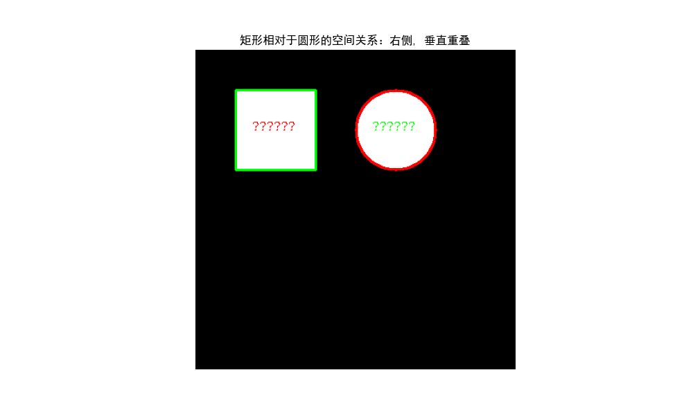
11.5 关系描述子

        关系描述子通过描述目标各部分之间的空间关系（如上下、左右、包含）来表征目标，常用的有语义网络、句法描述等。

完整代码（关系描述子）

import cv2
import numpy as np
import matplotlib.pyplot as plt

plt.rcParams['font.sans-serif'] = ['SimHei']
plt.rcParams['axes.unicode_minus'] = False

def spatial_relationship(contour1, contour2):
    """判断两个轮廓的空间关系"""
    # 计算轮廓的包围盒
    x1, y1, w1, h1 = cv2.boundingRect(contour1)
    x2, y2, w2, h2 = cv2.boundingRect(contour2)
    
    # 计算中心坐标
    cx1 = x1 + w1/2
    cy1 = y1 + h1/2
    cx2 = x2 + w2/2
    cy2 = y2 + h2/2
    
    # 判断关系
    relations = []
    # 水平关系
    if cx1 < cx2 - w2/2:
        relations.append("左侧")
    elif cx1 > cx2 + w2/2:
        relations.append("右侧")
    else:
        relations.append("水平重叠")
    
    # 垂直关系
    if cy1 < cy2 - h2/2:
        relations.append("上方")
    elif cy1 > cy2 + h2/2:
        relations.append("下方")
    else:
        relations.append("垂直重叠")
    
    # 包含关系
    if (x1 < x2 and y1 < y2 and x1 + w1 > x2 + w2 and y1 + h1 > y2 + h2):
        relations.append("包含")
    elif (x2 < x1 and y2 < y1 and x2 + w2 > x1 + w1 and y2 + h2 > y1 + h1):
        relations.append("被包含")
    
    return relations

def relational_descriptors_demo():
    """关系描述子演示"""
    # 1. 生成包含两个形状的测试图像
    img = np.zeros((400, 400, 3), dtype=np.uint8)
    # 绘制矩形
    cv2.rectangle(img, (50, 50), (150, 150), (255, 255, 255), -1)
    # 绘制圆形
    cv2.circle(img, (250, 100), 50, (255, 255, 255), -1)
    img_rgb = img.copy()
    
    # 2. 预处理
    gray = cv2.cvtColor(img, cv2.COLOR_BGR2GRAY)
    ret, binary = cv2.threshold(gray, 127, 255, cv2.THRESH_BINARY)
    contours, _ = cv2.findContours(binary, cv2.RETR_EXTERNAL, cv2.CHAIN_APPROX_SIMPLE)
    
    # 3. 分析空间关系（假设两个轮廓）
    if len(contours) >= 2:
        contour1 = contours[0]  # 矩形
        contour2 = contours[1]  # 圆形
        relations = spatial_relationship(contour1, contour2)
        
        # 4. 绘制结果
        img_relation = img_rgb.copy()
        cv2.drawContours(img_relation, [contour1], -1, (255, 0, 0), 2)
        cv2.drawContours(img_relation, [contour2], -1, (0, 255, 0), 2)
        
        # 添加文字说明
        cv2.putText(img_relation, '矩形', (70, 100), cv2.FONT_HERSHEY_SIMPLEX, 0.5, (255, 0, 0), 1)
        cv2.putText(img_relation, '圆形', (220, 100), cv2.FONT_HERSHEY_SIMPLEX, 0.5, (0, 255, 0), 1)
        
        # 5. 显示结果
        plt.figure(figsize=(10, 6))
        plt.imshow(img_relation)
        plt.title(f'矩形相对于圆形的空间关系：{", ".join(relations)}')
        plt.axis('off')
        plt.show()
        
        # 打印关系描述
        print("=== 关系描述子 ===")
        print(f"矩形相对于圆形的空间关系：{', '.join(relations)}")
    else:
        print("图像中至少需要两个目标轮廓！")

if __name__ == "__main__":
    relational_descriptors_demo()

小结

核心知识点总结

1. 表示方法：核心是将原始边界 / 区域转换为简洁形式（如链码、多边形、骨架），为描述做准备，边界跟踪是所有表示方法的基础；
2. 描述子分类：边界描述子（傅里叶描述子、形状数）侧重轮廓特征，区域描述子（Hu 矩、纹理）侧重区域整体属性，优秀的描述子应具备平移 / 旋转 / 尺度不变性；
3. 实用技巧：PCA 可用于特征降维，拓扑描述子（欧拉数）适合描述连通性，关系描述子适合多目标空间关系分析。

工程应用建议

1. 简单形状识别优先使用Hu 不变矩或傅里叶描述子，计算高效且鲁棒性强；
2. 纹理丰富的图像优先使用灰度共生矩阵（GLCM） 提取纹理特征；
3. 多目标场景可结合拓扑描述子和关系描述子分析目标间的结构关系。

注意事项

1. 运行代码前需安装依赖：pip install opencv-python numpy matplotlib scikit-image scikit-learn；
2. 建议准备测试图像（如test_shape.jpg、test_texture.jpg），或使用代码中自动生成的测试图像；