[机器学习]基于K-means聚类算法的鸢尾花数据及分类

基于Kmeans算法对鸢尾花数据集前两个特征进行聚类，并比对不同类别数的分析结果

CONDIMENTTTT

709人浏览 · 2025-08-29 15:25:28

CONDIMENTTTT · 2025-08-29 15:25:28 发布

基于Kmeans，对鸢尾花数据集前两个特征进行聚类分析

通过迭代优化，将150个样本划分到K个簇中。
目标函数：最小化所有样本到其所属簇中心的距离平方和。
算法步骤：
1. 随机初始化K个簇中心。
2. 将每个样本分配到最近的中心。
3. 计算均值确定每个簇的中心（均值）。
4. 重复第2和3步直到稳定收敛。

程序代码：

import math

import numpy as np
from matplotlib import pyplot as plt
from sklearn import datasets

plt.rcParams['font.sans-serif'] = ['SimHei']
plt.rcParams['axes.unicode_minus'] = False

data = datasets.load_iris().data
labels = datasets.load_iris().target
print('数据维度',data.shape)
features = data[:,: 2]
print('特征',features)

num_clusters = 6
epoch = 150
J_sum = []

def J_calculate(features,divide_re,center):
    J = 0
    for s1 in range(150):
        distances = ((features[s1][0]-center[divide_re[s1]][0]) ** 2) + ((features[s1][1]-center[divide_re[s1]][1]) ** 2)
        #print(distances)
        J = J + distances
    return J

def decision(features,divide_re,center,epoch):
    J_best = []
    for _ in range(epoch):
        J_b = math.inf
        for s1 in range(150):
            best = None
            min_J_now = math.inf
            for s2 in range(len(center)):
                divide_re[s1] = s2
                J_now = J_calculate(features,divide_re,center)
                if J_now < min_J_now:
                    min_J_now = J_now
                    best = s2
            divide_re[s1] = best
            for i in range(len(center)):
                xc = []
                yc = []
                for j in range(150):
                    if (divide_re[j] == i):
                        xc.append(features[j][0])
                        yc.append(features[j][1])
                center[i] = [np.mean(xc), np.mean(yc)]

            if(min_J_now<J_b):
                J_b = min_J_now
        J_best.append(J_b)

    return features,divide_re,center,J_best

for i in range(2,num_clusters+1):
    print(f'\n分{i}类:\n')
    center = features[np.random.choice(features.shape[0], i, replace=False)]
    print("初始中心点", center)
    distances = np.linalg.norm(features[:, np.newaxis, :] - center, axis=2)
    divide = np.argmin(distances,axis=1)
    divide_re = []
    for x in range(150):
        divide_re.append(divide[x])
    print("初始样本分类", divide_re)
    features,divide_re,center,J_best = decision(features,divide_re,center,epoch)
    print(f'{i}类最佳J值为:',J_best[epoch-1])
    J_sum.append(J_best[epoch-1])
    plt.scatter(features[:, 0], features[:, 1], c=divide_re, cmap='viridis', edgecolors='k')
    plt.scatter(center[:, 0], center[:, 1], marker='x', s=30, linewidths=3, color='red')
    plt.title(f'{i}类C均值分类法结果')
    plt.xlabel('第一特征')
    plt.ylabel('第二特征')
    plt.show()
plt.figure()
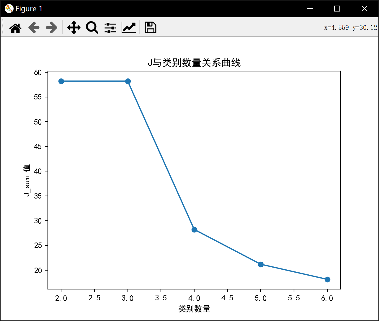
plt.plot(range(2, num_clusters + 1), J_sum, marker='o')
plt.title('J与类别数量关系曲线')
plt.xlabel('类别数量')
plt.ylabel('J_sum 值')
plt.show()

运行结果：

数据维度 (150, 4)
特征 [[5.1 3.5]
[4.9 3. ]
[4.7 3.2]
[4.6 3.1]
[5. 3.6]
[5.4 3.9]
[4.6 3.4]
[5. 3.4]
[4.4 2.9]
[4.9 3.1]
[5.4 3.7]
[4.8 3.4]
[4.8 3. ]
[4.3 3. ]
[5.8 4. ]
[5.7 4.4]
[5.4 3.9]
[5.1 3.5]
[5.7 3.8]
[5.1 3.8]
[5.4 3.4]
[5.1 3.7]
[4.6 3.6]
[5.1 3.3]
[4.8 3.4]
[5. 3. ]
[5. 3.4]
[5.2 3.5]
[5.2 3.4]
[4.7 3.2]
[4.8 3.1]
[5.4 3.4]
[5.2 4.1]
[5.5 4.2]
[4.9 3.1]
[5. 3.2]
[5.5 3.5]
[4.9 3.6]
[4.4 3. ]
[5.1 3.4]
[5. 3.5]
[4.5 2.3]
[4.4 3.2]
[5. 3.5]
[5.1 3.8]
[4.8 3. ]
[5.1 3.8]
[4.6 3.2]
[5.3 3.7]
[5. 3.3]
[7. 3.2]
[6.4 3.2]
[6.9 3.1]
[5.5 2.3]
[6.5 2.8]
[5.7 2.8]
[6.3 3.3]
[4.9 2.4]
[6.6 2.9]
[5.2 2.7]
[5. 2. ]
[5.9 3. ]
[6. 2.2]
[6.1 2.9]
[5.6 2.9]
[6.7 3.1]
[5.6 3. ]
[5.8 2.7]
[6.2 2.2]
[5.6 2.5]
[5.9 3.2]
[6.1 2.8]
[6.3 2.5]
[6.1 2.8]
[6.4 2.9]
[6.6 3. ]
[6.8 2.8]
[6.7 3. ]
[6. 2.9]
[5.7 2.6]
[5.5 2.4]
[5.5 2.4]
[5.8 2.7]
[6. 2.7]
[5.4 3. ]
[6. 3.4]
[6.7 3.1]
[6.3 2.3]
[5.6 3. ]
[5.5 2.5]
[5.5 2.6]
[6.1 3. ]
[5.8 2.6]
[5. 2.3]
[5.6 2.7]
[5.7 3. ]
[5.7 2.9]
[6.2 2.9]
[5.1 2.5]
[5.7 2.8]
[6.3 3.3]
[5.8 2.7]
[7.1 3. ]
[6.3 2.9]
[6.5 3. ]
[7.6 3. ]
[4.9 2.5]
[7.3 2.9]
[6.7 2.5]
[7.2 3.6]
[6.5 3.2]
[6.4 2.7]
[6.8 3. ]
[5.7 2.5]
[5.8 2.8]
[6.4 3.2]
[6.5 3. ]
[7.7 3.8]
[7.7 2.6]
[6. 2.2]
[6.9 3.2]
[5.6 2.8]
[7.7 2.8]
[6.3 2.7]
[6.7 3.3]
[7.2 3.2]
[6.2 2.8]
[6.1 3. ]
[6.4 2.8]
[7.2 3. ]
[7.4 2.8]
[7.9 3.8]
[6.4 2.8]
[6.3 2.8]
[6.1 2.6]
[7.7 3. ]
[6.3 3.4]
[6.4 3.1]
[6. 3. ]
[6.9 3.1]
[6.7 3.1]
[6.9 3.1]
[5.8 2.7]
[6.8 3.2]
[6.7 3.3]
[6.7 3. ]
[6.3 2.5]
[6.5 3. ]
[6.2 3.4]
[5.9 3. ]]

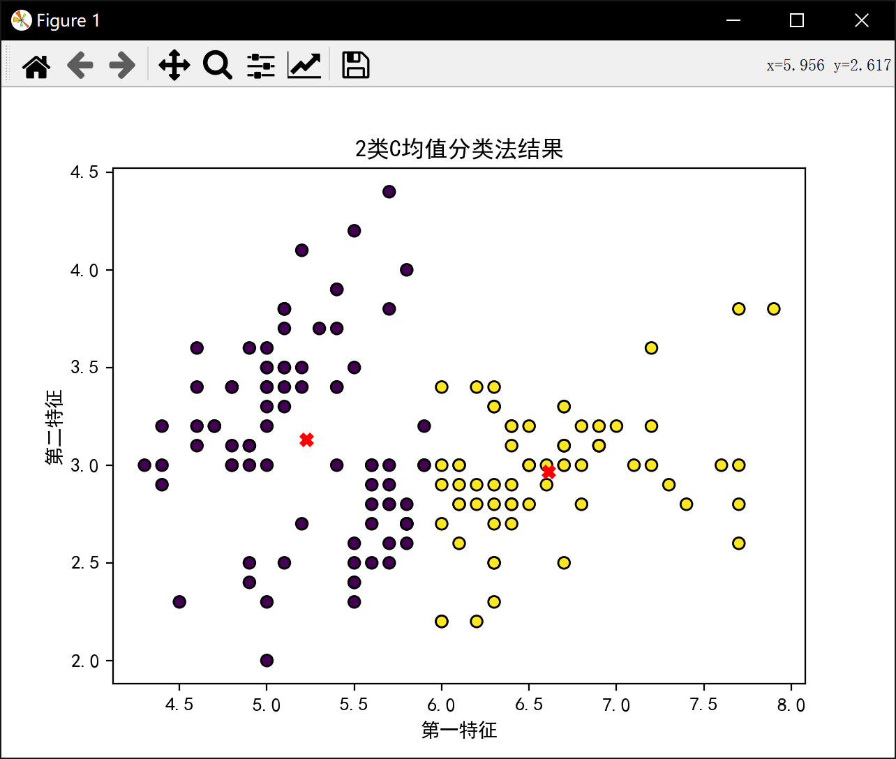
分2类:

初始中心点 [[6.4 3.1]
[7.2 3.6]]
初始样本分类 [0, 0, 0, 0, 0, 0, 0, 0, 0, 0, 0, 0, 0, 0, 0, 0, 0, 0, 0, 0, 0, 0, 0, 0, 0, 0, 0, 0, 0, 0, 0, 0, 0, 0, 0, 0, 0, 0, 0, 0, 0, 0, 0, 0, 0, 0, 0, 0, 0, 0, 1, 0, 0, 0, 0, 0, 0, 0, 0, 0, 0, 0, 0, 0, 0, 0, 0, 0, 0, 0, 0, 0, 0, 0, 0, 0, 0, 0, 0, 0, 0, 0, 0, 0, 0, 0, 0, 0, 0, 0, 0, 0, 0, 0, 0, 0, 0, 0, 0, 0, 0, 0, 1, 0, 0, 1, 0, 1, 0, 1, 0, 0, 0, 0, 0, 0, 0, 1, 1, 0, 1, 0, 1, 0, 0, 1, 0, 0, 0, 1, 1, 1, 0, 0, 0, 1, 0, 0, 0, 0, 0, 0, 0, 0, 0, 0, 0, 0, 0, 0]
2类最佳J值为: 58.20409278906674

分3类:

初始中心点 [[5.4 3.4]
[5.4 3.4]
[7.7 2.8]]
初始样本分类 [0, 0, 0, 0, 0, 0, 0, 0, 0, 0, 0, 0, 0, 0, 0, 0, 0, 0, 0, 0, 0, 0, 0, 0, 0, 0, 0, 0, 0, 0, 0, 0, 0, 0, 0, 0, 0, 0, 0, 0, 0, 0, 0, 0, 0, 0, 0, 0, 0, 0, 2, 0, 2, 0, 2, 0, 0, 0, 2, 0, 0, 0, 0, 0, 0, 2, 0, 0, 0, 0, 0, 0, 0, 0, 0, 2, 2, 2, 0, 0, 0, 0, 0, 0, 0, 0, 2, 0, 0, 0, 0, 0, 0, 0, 0, 0, 0, 0, 0, 0, 0, 0, 2, 0, 0, 2, 0, 2, 2, 2, 0, 0, 2, 0, 0, 0, 0, 2, 2, 0, 2, 0, 2, 0, 2, 2, 0, 0, 0, 2, 2, 2, 0, 0, 0, 2, 0, 0, 0, 2, 2, 2, 0, 2, 2, 2, 0, 0, 0, 0]

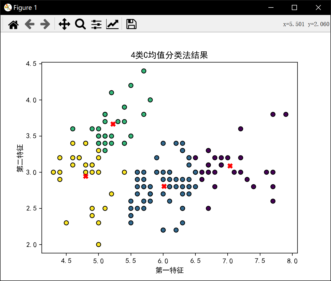
3类最佳J值为: 58.20409278906674

分4类:

初始中心点 [[6.7 3.1]
[6.4 2.7]
[6.5 3.2]
[5.5 2.4]]
初始样本分类 [3, 3, 3, 3, 3, 2, 3, 3, 3, 3, 2, 3, 3, 3, 2, 2, 2, 3, 2, 3, 3, 3, 3, 3, 3, 3, 3, 3, 3, 3, 3, 3, 2, 2, 3, 3, 2, 3, 3, 3, 3, 3, 3, 3, 3, 3, 3, 3, 2, 3, 0, 2, 0, 3, 1, 3, 2, 3, 0, 3, 3, 1, 3, 1, 3, 0, 3, 3, 1, 3, 2, 1, 1, 1, 1, 0, 0, 0, 1, 3, 3, 3, 3, 1, 3, 2, 0, 1, 3, 3, 3, 1, 3, 3, 3, 3, 3, 1, 3, 3, 2, 3, 0, 1, 2, 0, 3, 0, 1, 0, 2, 1, 0, 3, 3, 2, 2, 0, 0, 3, 0, 3, 0, 1, 0, 0, 1, 1, 1, 0, 0, 0, 1, 1, 1, 0, 2, 2, 1, 0, 0, 0, 3, 0, 0, 0, 1, 2, 2, 1]
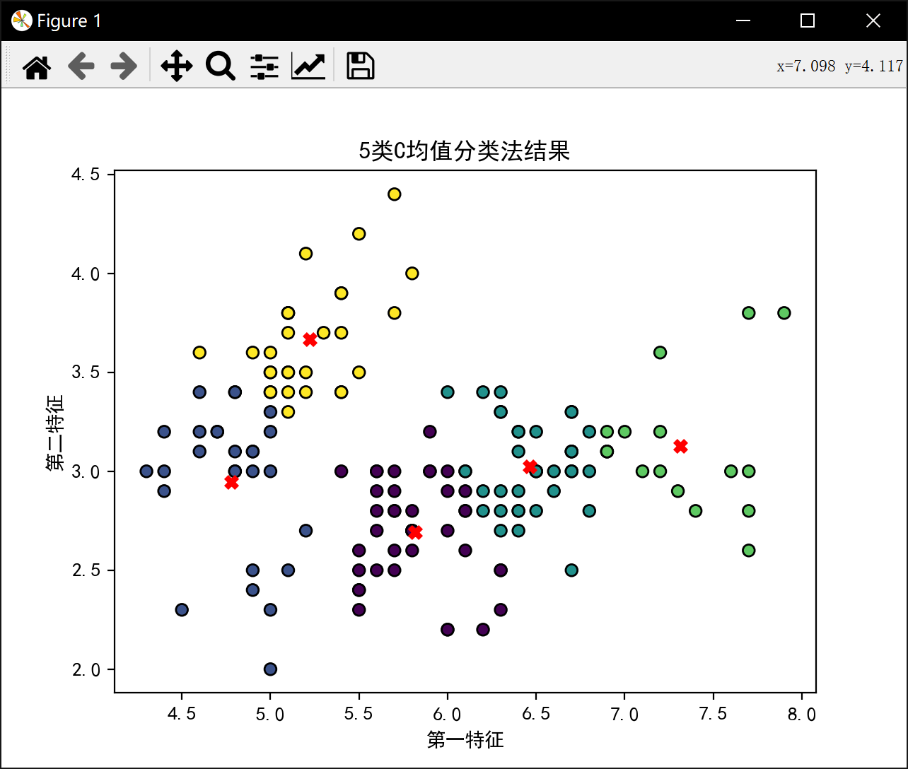
4类最佳J值为: 28.23339146670904

分5类:

初始中心点 [[6.3 2.5]
[5.1 3.5]
[6.4 3.2]
[7.1 3. ]
[5.5 3.5]]
初始样本分类 [1, 1, 1, 1, 1, 4, 1, 1, 1, 1, 4, 1, 1, 1, 4, 4, 4, 1, 4, 1, 4, 1, 1, 1, 1, 1, 1, 1, 1, 1, 1, 4, 1, 4, 1, 1, 4, 1, 1, 1, 1, 1, 1, 1, 1, 1, 1, 1, 1, 1, 3, 2, 3, 0, 0, 0, 2, 1, 2, 1, 0, 2, 0, 2, 4, 2, 4, 0, 0, 0, 2, 0, 0, 0, 2, 2, 3, 2, 0, 0, 0, 0, 0, 0, 4, 2, 2, 0, 4, 0, 0, 2, 0, 1, 0, 4, 4, 2, 1, 0, 2, 0, 3, 2, 2, 3, 1, 3, 0, 3, 2, 0, 3, 0, 0, 2, 2, 3, 3, 0, 3, 4, 3, 0, 2, 3, 0, 2, 0, 3, 3, 3, 0, 0, 0, 3, 2, 2, 2, 3, 2, 3, 0, 3, 2, 2, 0, 2, 2, 2]
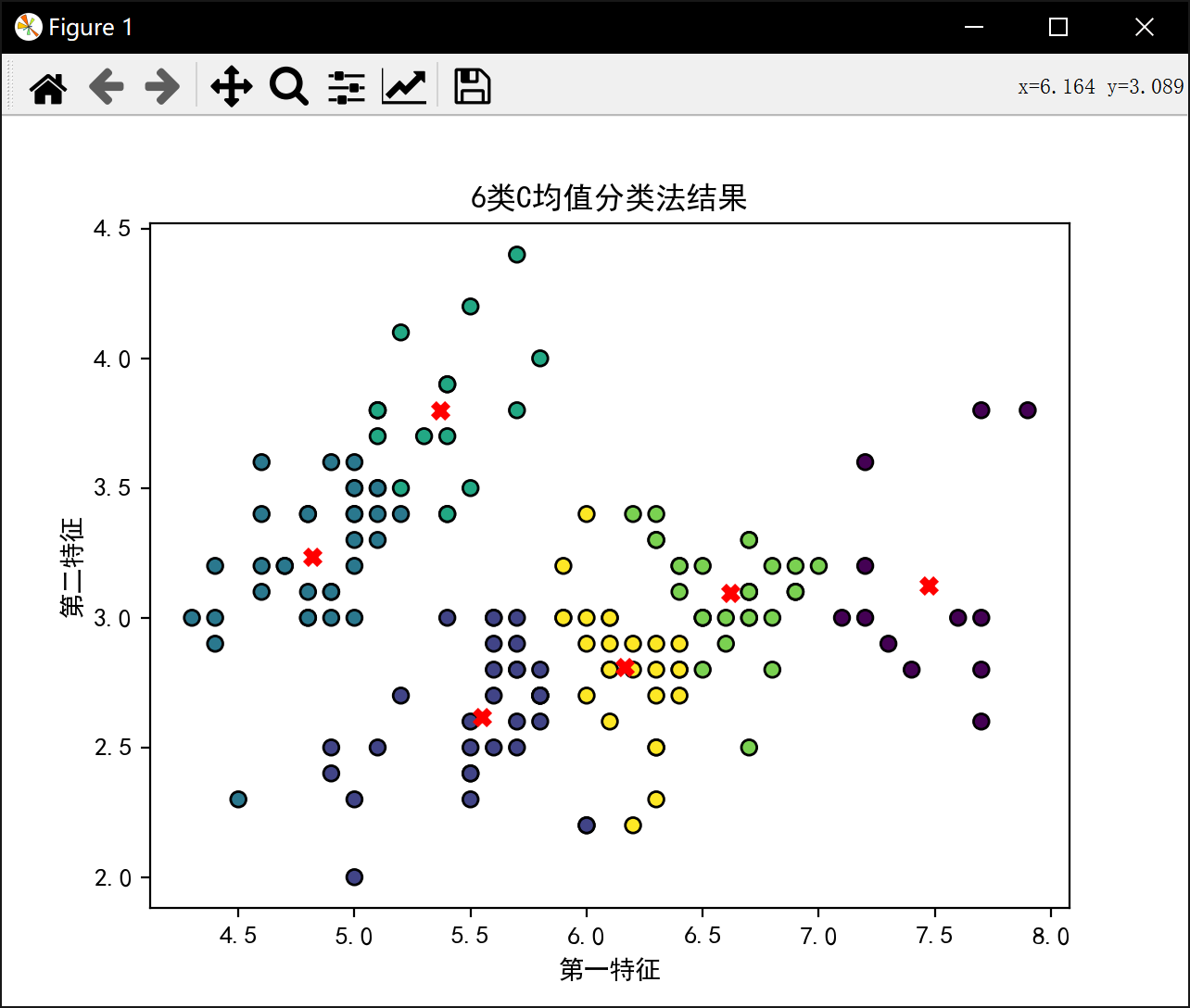
5类最佳J值为: 21.200013093214928

分6类:

初始中心点 [[6.8 2.8]
[5.8 2.6]
[4.4 3. ]
[6.2 3.4]
[6.4 3.2]
[6. 3. ]]
初始样本分类 [2, 2, 2, 2, 2, 3, 2, 2, 2, 2, 3, 2, 2, 2, 3, 3, 3, 2, 3, 2, 5, 2, 2, 2, 2, 2, 2, 2, 2, 2, 2, 5, 3, 3, 2, 2, 5, 2, 2, 2, 2, 2, 2, 2, 2, 2, 2, 2, 3, 2, 0, 4, 0, 1, 0, 1, 3, 2, 0, 1, 1, 5, 1, 5, 1, 4, 5, 1, 1, 1, 5, 5, 1, 5, 4, 4, 0, 0, 5, 1, 1, 1, 1, 1, 1, 3, 4, 1, 5, 1, 1, 5, 1, 1, 1, 5, 1, 5, 1, 1, 3, 1, 0, 5, 4, 0, 2, 0, 0, 4, 4, 0, 0, 1, 1, 4, 4, 0, 0, 1, 0, 1, 0, 5, 4, 0, 5, 5, 0, 0, 0, 0, 0, 5, 1, 0, 3, 4, 5, 0, 4, 0, 1, 4, 4, 0, 1, 4, 3, 5]
6类最佳J值为: 18.150987445152886

进程已结束,退出代码0